From RankNet to LambdaRank to LambdaMART: An Overview (Chris Burges)

Deriving lambda from pairwise cross-entropy

Problem: query $q$, documents $U_i$ and $U_j$. Predicted scores: $s_i=f(x_i)$

$U_i > U_j$ means $U_i$ should be ranked before $U_j$.

$P_{ij}=P(U_i > U_j)=\frac{1}{1+e^{-\sigma\times(s_i - s_j)}}$

where $\sigma$ is a scalar that determines the shape of the sigmoid.

Given relevance labels $l_i$ for each doc (1, 0 or -1), let $S_{ij}=1$ if $l_i > l_j$, $0$ if $l_i = l_j$ and $-1$ if $U_i < U_j$.

True probability: $P_{ij}^*=\frac{1}{2}(1+S_{ij})$

Cross-entropy cost: $C = P_{ij}=-P_{ij}^* \log (P_{ij}) - (1-P_{ij}^*)\log (1 - P_{ij}) = \frac{1}{2}(1-S_{ij})g(s_i - s_j) + \log (1+e^{-g(s_i - s_j)})$

If we take the derivative: $\frac{\partial C}{\partial s_i}=\sigma\times (s_i - s_j)[\frac{1}{2}(1-S_{ij})-\frac{1}{1+e^{\sigma\times(s_i - s_j)}}] = -\frac{\partial C}{\partial s_j}$

SGD update is: $w_k \leftarrow w_k - \eta \frac{\partial C}{\partial w_k}$

$\frac{\partial C}{\partial s_i}\frac{\partial s_i}{\partial w_k} + \frac{\partial C}{\partial s_j}\frac{\partial s_j}{\partial w_k} = \frac{\partial C}{\partial s_i}(\frac{\partial s_i}{\partial w_k} - \frac{\partial s_j}{\partial w_k}) = \lambda_{ij}(\frac{\partial s_i}{\partial w_k} - \frac{\partial s_j}{\partial w_k})$

Let $I$ denote indexes $i,j$ such that $U_i > U_j$. Therefore, $S_{ij}=1$ always.

Summing up all contributions to the update of weight $w_k$:

$\delta w_k = -\eta \sum_{(i,j)\in I}(\lambda_{ij} \frac{\partial s_i}{\partial w_k} - \lambda_{ij} \frac{\partial s_j}{\partial w_k}) = -\eta \sum_i \lambda_i \frac{\partial s_i}{\partial w_k}$ where $\lambda_i = \sum_{j:(i,j)\in I}\lambda_{ij} - \sum_{j:(j,i)\in I}\lambda_{ij}$

$\lambda_i$ is a force attached to doc $i$, the direction of which indicates the direction we would like the URLs to move (to increase relevance), and the length of which indicates by how much. It is comupted from all the pairs in which $i$ is a member.

SGD: weights are updated after each pair.

Instead, we can use mini-batch SGD and accumulate $\lambda$s.

This speeds up training from $\approx O(n^2)$ ($n$ = number of docs) to $\approx O(n)$

Optimizing information retrieval measures

IR measures as a function of model scores are discontinuous or flat. Thus, gradients are zero or undefined.

Expected reciprocal rank (inspired by a cascade model where user scrolls until it finds a result):

$ERR=\sum_{r=1}^n \frac{1}{r} R_r \prod_{i=1}^{r-1} (1- R_i)$

where $R_i=\frac{2^l_i - 1}{\max l_i}$ is the prob that user finds item $i$ relevant.

ERR is the expected proba to arrive at relevant item over the result length.

RankNet is optimizing a smooth, convex approximation of the number of pairwise errors (since cross-entropy penalizes $s_i - s_j$)

Explanation in the Lambdarank paper:

Suppose that a ranking algorithm $A$ is being trained, and that at some iteration, for a query for which there are only two relevant documents $D_1$ and $D_2$, A gives $D_1$ rank one and $D_2$ rank $n$. Then on this query, $A$ has WTA (winner takes all) cost zero, but a pairwise error cost of $n − 2$ (since $D_2$ is higher than docs at position $2, 3, ..., n-1$. If the parameters of A are adjusted so that $D_1$ has rank two, and $D_2$ rank three, then the WTA error is now maximized (=1), but the number of pairwise errors has been reduced by $n − 4$. Now suppose that at the next iteration, $D_1$ is at rank two, and $D_2$ at rank $n$ ≫ 1. The change in $D_1$’s score that is required to move it to top position is clearly less (possibly much less) than the change in $D_2$’s score required to move it to top position. Roughly speaking, we would prefer $A$ to spend a little capacity moving $D_1$ up by one position, than have it spend a lot of capacity moving $D_2$ up by $n − 1$ positions.

Cross-entropy doesn't make this distinction. It minimizes the pairwise number of errors. Rather than deriving gradients from a cost, it would be easier to write them down directly.

The forces $\lambda$s are exactly those gradients. Experiments show that simply multiplying $\lambda_{ij}$ by $\lvert \Delta_{NDCG}\rvert$, the NDCG change by swapping position $i$ and $j$ gives very good results. In LambdaRank, we imagine that there is a utility $C$ such that (recall that $S_{ij} = 1$):

$\lambda_{ij}=\frac{-\sigma}{1+e^{g(s_i - s_j)}}\lvert \Delta_{NDCG}\rvert$

Although information retrieval measures, viewed as a function of scores are flat/discontinuous, LambdaRank bypasses this problem by computing gradients after docs have been sorted. Thanks to the $\Delta_{NDCG}$ value, we can give more importance to earlier ranks.

Every document pair generates an equal and opposite $\lambda$, and for a given document, all the lambdas are incremented (from contributions from all pairs in which it is a member, where the other member of the pair has a different relevance label). This accumulation is done for every document for a given query; when that calculation is done, the weights are adjusted based on the computed lambdas using a small (stochastic gradient) step. This speeds up training.

Empirical optimization of NDCG

Empirically, such a model optimizes NDCG directly. To optimize other metrics, just change $\lvert \Delta_{NDCG}\rvert$ into the appropriate measure.

Let $M$ be the average NDCG of our model over all queries. By fixing every parameter except one $w_i$, we can define some gradient: $\frac{\partial M}{\partial w_i} = \frac{M - M^*}{w_i-w_i^*}$ where $w_i^*$ is the learned parameter. As $w_i$ changes, this gradient resembles little step functions.

We want to show that $w_i^*$ is a local maximum. Computing the Hessian is too computationally challenging, so instead, we choose sufficiently many random directions in weight space and check that $M$ is decreasing as we move away from the learned weights $w^*$. They derive some p-value of missing an ascent direction (it's a one-sided Monte-Carlo test) to choose the minimum number of directions required.

*Can we always find a cost such that arbitrary $\lambda$s are its gradient?

Poincarré's Lemma states that $f_1(x_1, \dots, x_n), f_2(x_1,\dots, x_n), \dots$ are partial derivatives of some function $F$ (i.e. $\frac{\partial F}{\partial x_i} = f_i$) iff $\frac{\partial f_i}{\partial x_j} = \frac{\partial f_j}{\partial x_i} \forall (i,j)$

Application to MART (binary classification)

MART = gradient boosting (see notes on the gradient boosting paper)

Quick recap:

Final model is a linear combination of weak learners: $F(x)=\sum_{m=1}^M \beta_m h(x; a_m)$

where $\beta_m$ and $a_m$ are learned in a greedy stagewise manner:

$\beta_m, a_m = \arg\min \sum_{i=1}^N L(y_i; F_{m-1}(x_i))$

The update is then: $F_m(x)=F_{m-1}(x) + \beta_m h(x; a_m)$

Descent direction is the gradient: $-g_m=-\big[ \frac{\partial L(y_i, F(x_i))}{\partial F(x_i)} \big]_{F(x)=F_{m-1}(x)}$

This gives the steepest descent in N dimensional data space at $F_{m-1}(x)$ but it's only defined at data points $x_i$ and cannot be generalized to other $x$. We take the closest least square estimate $a_m=\arg\min_{a,\beta} \sum [-g_m -\beta h(x_i; a)]^2$ and use line search.

$\beta_m = \arg\min_{\beta} \sum L(y_i, F_{m-1}(x)+\beta h(x))$

Base learner is a tree with $J$ terminal nodes:

$h(x)=\sum_{j=1} b_j \mathbb{I}(x\in R_j)$

where ${R_j}_{j=1}^J$ is a disjoint partition of $x$.

$F_m(x)=F_{m-1}(x)+\beta_m \sum_{j=1}^J b_{jm}\mathbb{I}(x\in R_{jm})=F_{m-1}+\sum \gamma_{jm}\mathbb{I}(x\in R_{jm})$

where $\gamma_{jm}=\beta_m b_{jm}$

Since $R_j$ are disjoint, we can optimize each $\gamma_{jm}$ independently:

$\gamma_{jm}=\arg\min_{\gamma} \sum_{x_j\in R_{jm}}L(y_i, F_{m-1}(x_i) + \gamma)$

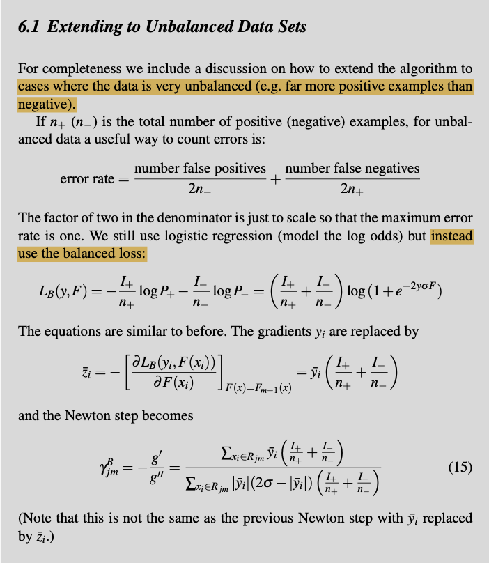
For binary classification, we take a Newton step since there is no closed form solution to $L(x)=\log(1+e^{-2F(x)})$:

$\gamma_{n+1}=\gamma_n - \frac{g'(\gamma_n)}{g''(\gamma_n)}$

where $g$ is the loss we're optimizing: $g(\gamma)=\sum_{x_j\in R_{jm}}\log(1+e^{-2F_{m-1}(x_i)+\gamma})$

This can be expressed with respect to the pseudoresponses:

$\bar{y_i}=-\big[\frac{\partial L(y_i, F(x_i))}{\partial F(x_i)}\big]_{F(x)=F_{m-1}(x)}$

These are the exact analogs to the Lambda gradients. We can specify the pseudo-responses (lambdas) directly to move $F_m$ in a certain direction.

The $\lambda_{ij}$s are defined as:

$\lambda_{ij}=\frac{-\sigma \lvert \Delta Z_{ij}\rvert}{1+e^{\sigma\times(s_i-s_j)}}$

We can find the cost for which they are the derivative: $C=\sum_{j:(i,j)\in I}\lvert \Delta Z_{ij}\rvert \log(1+\exp(\sigma(s_i-s_j)))-\sum_{j:(j,I)\in I}\lvert \Delta Z_{ij}\rvert \log(1+\exp(\sigma(s_i-s_j)))$

The pseudo-responses are then just $\partial C/\partial s_i$

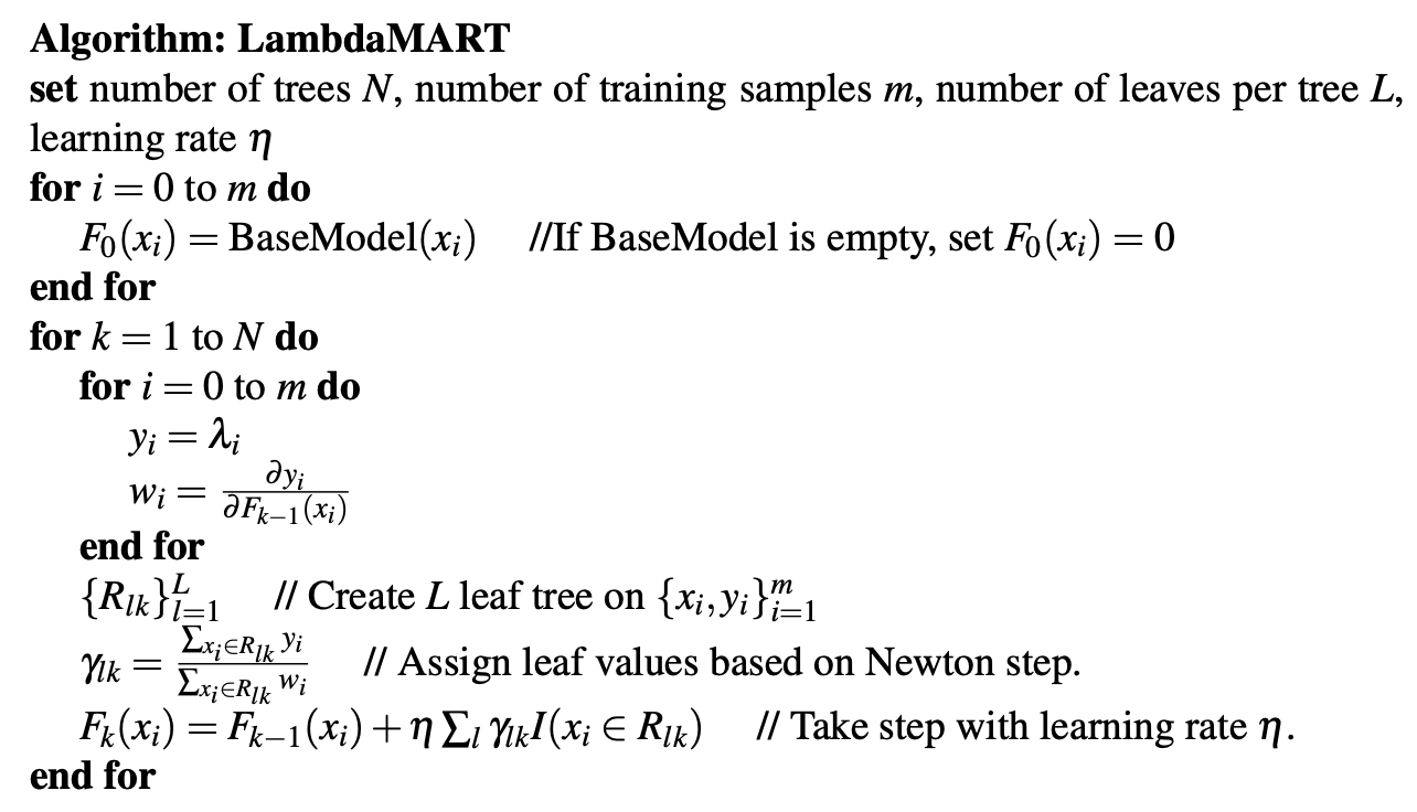
It’s useful to compare how LambdaRank and LambdaMART update their parameters. LambdaRank updates all the weights after each query is examined. The decisions (splits at the nodes) in LambdaMART, on the other hand, are computed using all the data that falls to that node, and so LambdaMART updates only a few parameters at a time (namely, the split values for the current leaf nodes), but using all the data (since every $x_i$ lands in some leaf). This means in particular that LambdaMART is able to choose splits and leaf values that may decrease the utility for some queries, as long as the overall utility increases.