paper (2015)

• Used as backbone for stable diffusion.
• Originally designed for image segmentation: a class label is assigned to each pixel.
• Leveraging data augmentation using elastic deformations, it needs few annotated images (30) to achieve best performance on biomedical segmentation (as of 2015) and has a training time of 10 hours on a NVidia Titan GPU (6 GB).
• It uses a contracting path to capture context and a symmetric, expanding path for precise localization.

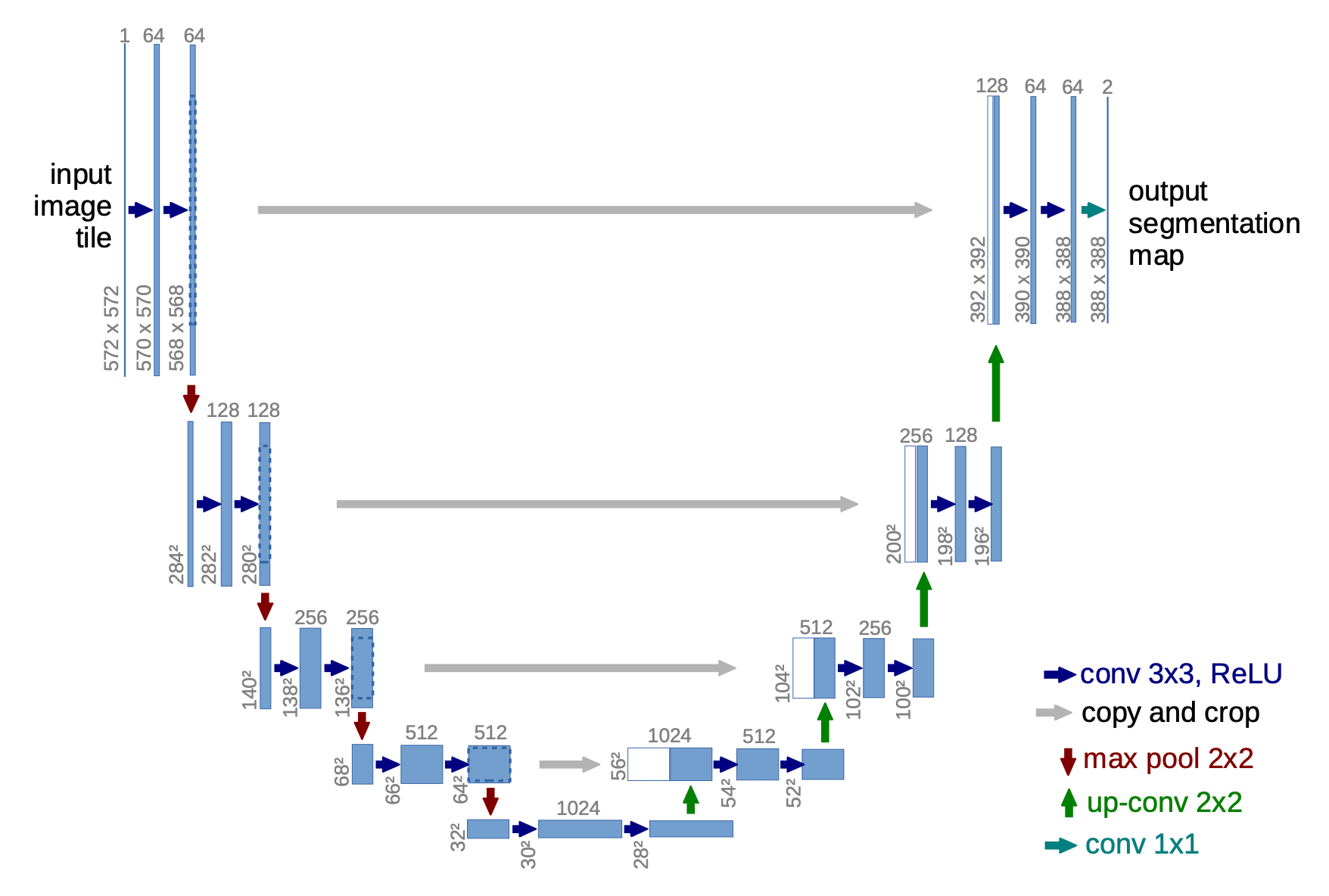
Architecture

For a recap on convolutions and up-convolutions, see the last section.

The architecture consists in:

• a contracting path (left side) is a typical convolutional network: repeated application of two $3\times 3$ unpadded convolutions, followed by ReLU and $2\times 2$ max-pooling with stride $2$ for downsampling. The number of feature channels is doubled at each convolution step, this ensures that as resolution decreases, the feature space's information capacity grows, avoiding bottlenecks.
• an expanding path (right side): every step consists of an upsampling of the feature map followed by a $2\times 2$ convolution ("up-convolution") that halves the number of feature channels, a concatenation with the cropped feature map from the contracting path and two $3\times 3$ convolutions, each followed by a ReLU. Cropping is necessary due to the loss of border pixels in every convolution.
• final layer: $1\times 1$ convolution is used to map each 64-component feature vector to the desired number of classes.
• There are no fully-connected layer in the architecture.

The loss function is the cross-entropy with respect to the soft-max over the classes for each pixel.

where:

• $w(x)$ is some weight map introduced to give some pixels more importance in the training
• $l(x)$ is the true class of pixel $x$, meaning $p_{l_x}(x)$ is the soft-max probability of class $l_x$

The weight map is pre-computed for each ground truth segmentation. The goal is to:

• compensate the different frequency of pixels within a certain class in the training set
• force the network to learn the small separation borders that we introduce between touching cells (by applying a large weight to this border). The goal is to separate touching objects of the same class.

where:

• $w_c$ is the weight map to balance class frequencies
• $d_1$ is the distance to the border of the nearest cell
• $d_2$ is the distance to the border of the second nearest cell

The layers are initialized such that each feature map has approximately unit variance (drawing initial weights from a Gaussian distribution with standard deviation of $\sqrt{2/N}$ where $N$ is the number of incoming nodes of one neuron).

Data augmentation

We need robustness to shift and rotation invariance. Applying random elastic deformations of the training samples allow them to use very few annotated images.

Recap on convolutions and up-convolutions

Convolution Operator

source

A 2D convolution is described by its kernel weights and the number of channels. The above figure shows just 1 channel.

Each output channel $c_{out}$, sums over all the input channels $c_{in}$. If we only look at 1 output channel, there is one weight matrix for each input channel. Each weight matrix is convoluted over its respective channel and summed.

Each output channel has its own set of weight matrices.

Denoting $x$ as the input image (with multiple channels), $w$ the 4D kernel, $b$ a bias term for output channel $c_{out}$:

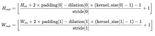
The output size of $y$ depends on the kernel size, stride and dilation:

(pytorch doc)

Up-convolution operator

Also referred to as "transposed convolutions" or "deconvolutions".

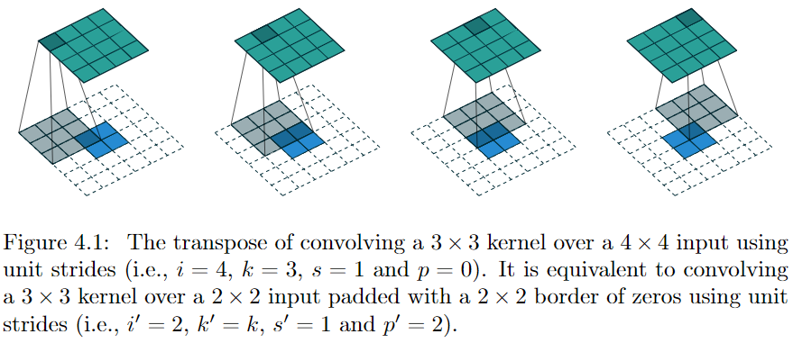
It consists in:

• padding the input feature map with zeros.
• applying a standard convolution on the padded map.