Imitation learning

Problem of learning policies from rewards is that rewards are often sparse. This is undesirable when data gathering is slow, costly or failure must be avoided.

One approach is to manually design reward functions that are dense in time. However, this requires a human to hand-design a reward function with the desired behavior in mind. It is thus desirable to learn by imitating agents.

Behavioral cloning

learn teacher's policy using supervised learning

Fix policy class and learn policy mapping states to actions given data tuples $\{(s_0, a_0), (s_1, a_1)\}$.

e.g.: ALVINN (map sensor inputs to steering angles)

Challenge: data not i.i.d. in state space. Trajectories are tightly clustered around expert trajectories. If a mistake is made that puts the agent in an unexplored state space, the errors compound quadratically (as opposed to linearly in standard RL). because each state has uniform probability of appearing?

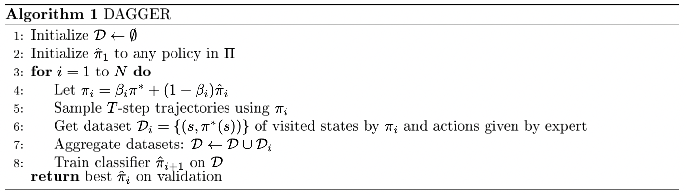
DAGGER: Dataset Aggregation

Mitigate problem of compounding errors by adding data for newly visited states. We assume that we can generate more data from an expert.

Inverse Reinforcement Learning

recover the reward function

Linear feature reward: $R(s)=w^T x(s)$

Resulting value function: $V^\pi(s)=\mathbb{E}_\pi[\sum_{t=0}^\infty \gamma^t R(s_t)\vert s_0=s]=w^T \underbrace{\mathbb{E}[\sum \gamma^t x(s_t)\vert s_0=s]}_{\mu(\pi\vert s_0=s)}$

where $\mu$ is the discounted weight frequency of state features $x(s)$ under $\pi$.

Under the optimal reward function, the export policy should have higher state values than the other ones. We want to find a paramterization of the reward function such that the expert policy outperforms other policies: $w^{*T} \mu(\pi^* \vert s_0=s)\geq w^{*T} \mu(\pi\vert s_0=s)$

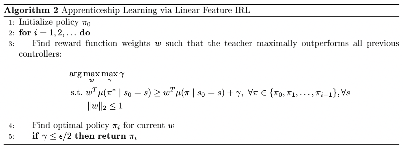
Apprenticeship Learning

use recovered rewards to generate a good policy

For policy $\pi$ to perform as well as expert policy $\pi^*$, it suffices that its discounted summed feature expectations match the expert's policy: $\lVert \mu(\pi\vert s_0=s) - \mu(\pi^*\vert s_0=s) \rVert_1 \leq \epsilon$

For policy $\pi$ to perform as well as expert policy $\pi^*$, it suffices that its discounted summed feature expectations match the expert's policy: $\lVert \mu(\pi\vert s_0=s) - \mu(\pi^*\vert s_0=s) \rVert_1 \leq \epsilon$

$\lVert w\rVert_\infty \leq 1$ + Cauchy-Schwartz ineq. $\Rightarrow \lVert w^T\mu(\pi\vert s_0=s) - w^T\mu(\pi^*\vert s_0=s) \rVert_1 \leq \epsilon$ why?

which optimization algo?

see Apprenticeship learning via inverse reinforcement learning

Maximum Entropy Inverse RL

TODO