Deep Q learning

Deep Q-Network (DQN): generalization

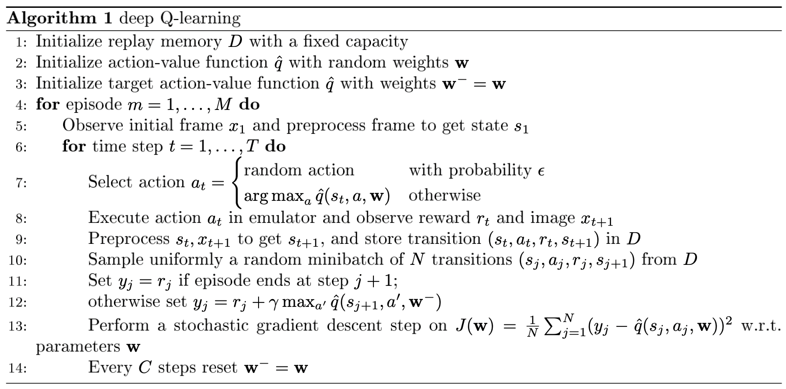
Playing Atari with Deep Reinforcement Learning (DeepMind, 2013)

Handcrafting an appropriate set of features doesn't scale up. deep neural nets enable automatic feature extractions.

DQN takes preprocessed pixel images from Atari game environment as inputs and outputs a vector containing Q-values for each valid action.

Preprocessing

raw Atari frames (210x160x3) are converted to gray scale and down-sampled to a 110x84 image, then cropped to a 84x84 region of the image capturing the play area (because of 2D convolutions expecting square input). 4 last frames are stacked to produce the input of size 84x84x4.

Architecture

• input = 84x84x4
• 1 convolution layer, 16 filters of size 8x8, stride 4 + ReLU
• 1 convolution layer, 32 filters of size 4x4, stride 2 + ReLU
• fully connected layer with size 256 + ReLU
• output layer is a fully connected linear layer (logits)

Training objective

$J(w)=\mathbb{E}_{(s_t,a_t,r_t,s_{t+1})}[(y_t^{DQN} - \hat q(s_t, a_t, w))^2]$

where $y_t^{DQN}$ is the one-step ahead learning target:

$y_t^{DQN} = r_t + \gamma \max_{a'}\hat q(s_{t+1}, a', w^-)$

where $w^-$ are the parameters of the target network and $w$ are the parameters of the online network.

Experience replay

Transition tuples $e_t = (s_t, a_t, r_t s_{t+1})$ are stored in a replay buffer $D_t=\{e_1, \dots, e_t\}$ used to store the most recent 1 million experiences. Online parameters $w$ are updated by sampling gradients uniformly from the mini-batch.

Learning directly from consecutive samples is inefficient, due to the strong correlations between the samples; randomizing the samples breaks these correlations and therefore reduces the variance of the updates.

When learning on-policy the current parameters determine the next data sample that the parameters are trained on. For example, if the maximizing action is to move left then the training samples will be dominated by samples from the left-hand side; if the maximizing action then switches to the right then the training distribution will also switch. It is easy to see how unwanted feedback loops may arise and the parameters could get stuck in a poor local minimum, or even diverge catastrophically.

When learning by experience replay, it is necessary to learn off-policy (because our current parameters are different to those used to generate the sample), which motivates the choice of Q-learning.

However, uniform sampling does not differentiate informative transitions. More sophisticated replay strategy: Prioritized Replay (replays important transitions more frequently = higher efficiency).

Has to be used with an off-policy method since the current parameters are different from those used to generate the samples.

Target network

To deal with non-stationary learning targets, the target network is used to generate targets $y_j$. Its parameters $w^-$ are updated every $C=10000$ steps by copying parameters from the online network. This makes learning more stable.

Training details

• reward clipping between -1 and 1 makes it possible to use the same learning rate across al different games.
• frame-skipping (or action repeat): the agent selects actions on every 4-th frame instead of every frame and its last action is repeated on skipped frames. Doesn't impact performance much and enables the agent to play roughly 4 times more games during training.
• RMSProp was used with minibatches of size 32. $\epsilon$-greedy policy with $\epsilon$ annealed from 1.0 to 0.1 over first million steps and fixed to 0.1 after. At eval time, $\epsilon=0.05$.

Double Deep Q-Network (DDQN): reducing maximization bias

max operator in DQN (line 12) uses same network values to select and evaluate an action, which causes maximization bias (likely to select overestimated values, resulting in overoptimistic target value estimates).

We decouple action selection parameters $w$ and action evaluation parameters $w'$:

$y_t^{DoubleQ}=r_t + \gamma \hat q(s_{t+1}, \arg\max_{a'} \hat q(s_{t+1}, a', w), w')$

We use the target network's parameters for evaluation: $w'=w^{-}$.

Dueling Network: decoupling value and advantage

Advantage function: $A^\pi(s,a)=Q^\pi(s,a) - V^\pi(s)$

Since $\mathbb{E}_{a\sim \pi}[Q^\pi(s,a)] = V^\pi(s)$, $\mathbb{E}[A^\pi(s,a)]=0$, meaning the advantage function is a relative measure of the importance of each action.

The dueling network learns the Q-function by decoupling value function and advantage function.

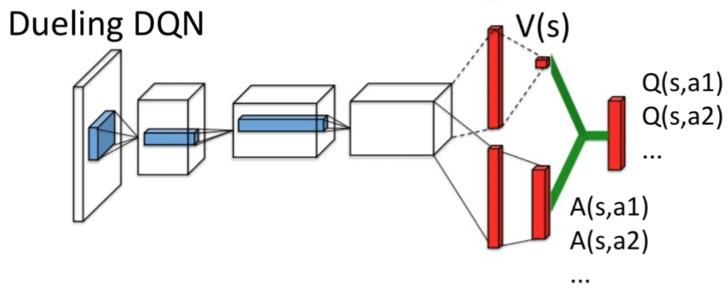
2 streams of fully connected layers:

• one provides value function estimates given state
• one estimates the advantage function for each valid action

Intuition:

• for many states, action selection has no impact on next state. However, state value estimation is important for every state for a bootstrapping based algorithm like Q-learning.
• features required to determine the value function may be different than those used to estimate action benefits

How to combine the two streams?

Just summing up $\hat q(s,a) = \hat v(s) + A(s,a)$ is unidentifiable (given $\hat q$ we cannot recover $\hat v$ or $A$: adding and subtracting any constant from the two values yields the same Q-value estimate). This also produces poor performance in practice.

For a deterministic, since we always choose the action $a^*=\arg\max_{a'}Q(s,a')$, $Q(s,a^*)=V(s)$ and hence $A(s,a^*)=0$. We can thus force the advantage function to have zero estimate at the chosen action:

$\hat q(s,a) = \hat v(s) + (A(s,a) - \max_{a'} A(s,a'))$

An alternative is to replace the max with a mean operator. This improves the stability of learning: the advantages only need to change as fast as the mean.