Model Free Control

• when MDP model is unknown but we can sample trajectories from the MDP, or
• when MDP model is known but computing value function via model-based control method is untractable

In policy iteration, we take $\pi^*(s)\leftarrow \arg\max_{a\in A}[R(s,a) + \gamma \sum_{s'\in S}P(s'\vert s,a)V^\pi(s')]$ but we can replace it with $Q^\pi(s,a)=R(s,a) + \gamma \sum_{s'\in S}P(s'\vert s,a)V^\pi(s')$ which is the discounted sum of returns, starting from state $s$ and taking action $a$.

Policy $\pi$ needs to take every action $a$ with some positive probability, so that we can compute the value of each state-action pair.

$\epsilon$-greedy policy with respect to state-action value $Q^\pi(s,a)$:

$\pi(a\vert s) = a \text{ with prob} \frac{\epsilon}{\lvert A \rvert}, \arg\max_a Q^\pi(s,a) \text{ with prob } 1-\epsilon$

We can show that the $\epsilon$-greedy policy $\pi_{i+1}$ with respect to $Q^{\pi_{i}}$ is a monotonic improvement on policy $\pi_i$, meaning $V^{\pi_{i+1}} \geq V^{\pi_i}$. See page 3, didn't understand the proof.

greedy in the limit of exploration (GLIE):

1. all state-action pairs are visited an infinite number of times

2. policy converges to the policy that is greedy with respect to the learned Q-function: $\lim_{i\to\infty} \pi_i(a\vert s)=\arg\max_a q(s,a) \text{ with prob } 1$

One example is $\epsilon$ decaying to zero with $\epsilon_i = 1/i$ ($i$ is the episode number).

Monte Carlo Control

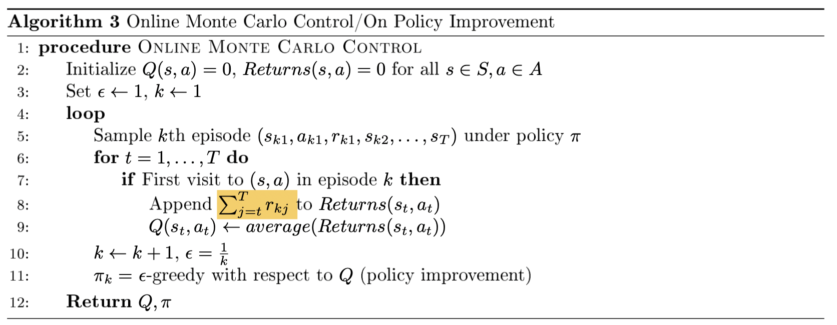
If the $\epsilon$-greedy strategy is GLIE then the Q value derived will converge to the optimal Q function.

Temporal Difference Methods

SARSA: on-policy

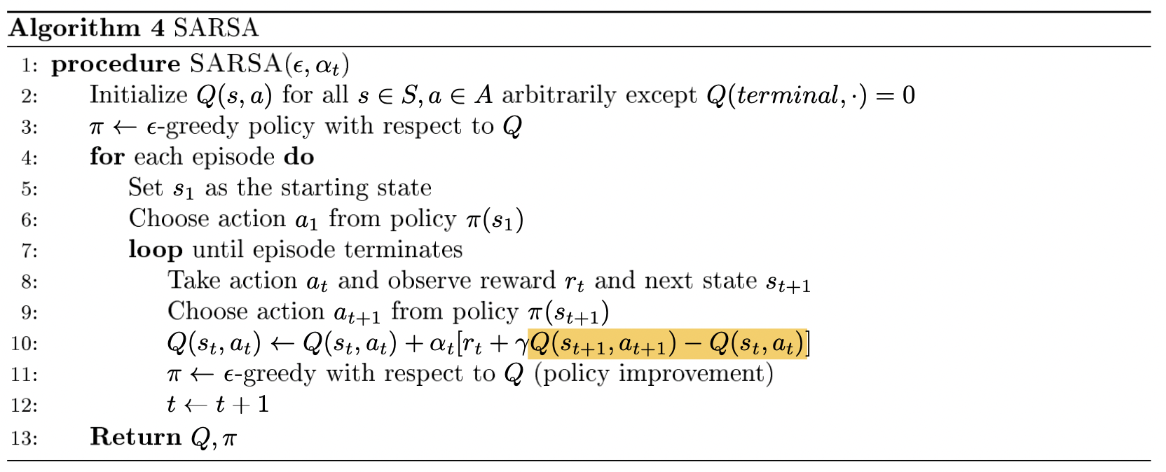
Called SARSA because we're using the values $(s,a,r,s',a')$ derived from the same policy.

SARSA converges to optimal Q if:

1. sequence of policies $\pi$ is GLIE

2. step-sizes $\alpha_t$ satisfy the Robbins-Munro sequence such that $\sum_{t=1}^\infty \alpha_t = \infty$ and $\sum_{t=1}^\infty \alpha_t^2 < \infty$

Q: how do you choose action $a_{t+1}$? If we just take the arg max, isn't it Q learning?

No: the action is chosen with an espilon greedy policy.

Importance sampling: off-policy

$V(s)\leftarrow V(s) + \alpha(r+\gamma V(s') - V(s))$ becomes $V^{\pi_e}(s)\leftarrow V^{\pi_e}(s) + \alpha [\frac{\pi_e(a\vert s)}{\pi_b(a\vert s)}(r+\gamma V^{\pi_e}(s') - V^{\pi_e}(s)]$

We only use one sample vs the entire trajectory like in Monte Carlo. Thus has significantly lower variance than Monte Carlo.

Q-learning: off-policy

SARSA update took the form:

$Q(s_t,a_t) \leftarrow Q(s_t,a_t) + \alpha_t[r_t + \gamma Q(s_{t+1}, a_{t+1}) - Q(s_t, a_t)]$

but we can bootstrap the Q value at the next state:

$Q(s_t,a_t)\leftarrow Q(s_t,a_t) + \alpha_t[r_t +\gamma\max_{a'}Q(s_{t+1}, a')-Q(s_t, a_t)]$

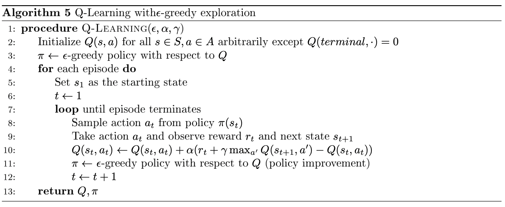
Q-learning always assumes optimal behavior in the future, even while the agent is still learning. SARSA uses the actual next action taken by the policy (which may be exploratory if it's epsilon-greedy), while Q-learning uses the best possible next action according to the current Q estimate.

Why is Q-learning off-policy and SARSA on policy?

The reason that Q-learning is off-policy is that it updates its Q-values using the Q-value of the next state $s'$ and the greedy action $a'$. In other words, it estimates the return (total discounted future reward) for state-action pairs assuming a greedy policy were followed despite the fact that it's not following a greedy policy.

The reason that SARSA is on-policy is that it updates its Q-values using the Q-value of the next state $s'$ and the current policy's action $a''$. It estimates the return for state-action pairs assuming the current policy continues to be followed.

The distinction disappears if the current policy is a greedy policy. However, such an agent would not be good since it never explores.

Double Q-learning

maximization bias appears when we are using our estimate to both choose the better action and estimate its value. (See coin example p.7)

Suppose two actions $a_1, a_2$ have mean reward $0$. We have $Q(s,a_1)=Q(s,a_2)=V(s)=0$. Suppose we estimated state-action values via Monte-Carlo: $\hat Q(s,a_i)=\frac{1}{n(s,a_i)}\sum_{j=1}^{n(s,a_i)}r_j(s,a_i)$. Let $\hat \pi=\arg \max_a \hat Q(s,a)$ be the greedy policy w.r.t. our estimates. Thus:

$\hat V(s)=\mathbb{E}[\max(\hat Q(s,a_1), \hat Q(s,a_2))] \geq \max(\mathbb{E}[\hat Q(s,a_1)],\mathbb{E}[\hat Q(s,a_2)]) = \max(0,0)=0=V^*(s)$

by Jensen's inequality and since each estimate is unbiased.

Therefore, we're systematically overestimating the value of the state.

We can get rid of this bias by decoupling the max and estimating the value of the max. We maintain two independent unbiased estimates $Q_1$ and $Q_2$. When we use one to select the maximum, we can use the other to get an estimate of the value of this maximum.

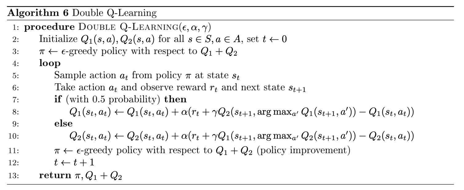
where we take the $\arg\max$ over $Q_1(s,a) + Q_2(s,a)$.

Double Q-learning can significantly speed up training because it eliminates suboptimal actions faster.