Model Free Evaluation

• we don't know the transition probabilities and rewards
• assume infinite horizon, stationary rewards, transition probabilities and policies

In dynamic programming, we bootstrap/estimate the value of the next state value using our current estimate $V_{k-1}(s')$ until convergence.

Monte-Carlo on-policy evaluation

Works for episodic environments.

1. Sample lots of episodes $h_j$ until termination

2. go over the episodes and keep track of:

   • $N(s)$: number of times we were in each step

   • $S(s)$: sum of total returns starting from the current step (e.g. for episode $j$, timestep $t$, $S(s_{j,t}) += G_t = \sum_{i=t}^{\lvert h_j\rvert} \gamma^{i-t}r_i$)

3. For each state $s$, $V(s)=S(s)/N(s)$

We can also keep an incremental estimate of $V(s)$:

$V(s) = V(s) + \underbrace{\frac{1}{N(s)}}_{\alpha}(G_t - V(s))$

When $\alpha > 1/N$, it gives higher weight to newer data, which helps in non-stationary settings.

Two variations:

• first-visit monte carlo (only update sate counters the first time we visit the state within the episode)
• every-visit monte carlo (more data efficient in a true Markovian setting)

Monte-Carlo off-policy evaluation

off-policy = use data taken from one policy to evaluate another

in costly or high stake situations we are not able to obtain rollouts of $G_t$ under the new policy.

Importance sampling

$\mathbb{E}_{x\sim q}[f(x)] = \int_x q(x)f(x)dx = \int_x p(x)\frac{q(x)/p(x)}f(x)dx = \mathbb{E}_{x\sim p}[\frac{q}{p}f]$

In our case $p = \pi_1$, the new policy we want to evaluate and $q = \pi_2$, the old policy under which the episodes were generated.

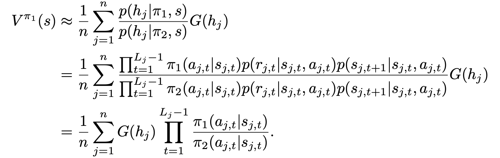
where $G(h_j)$ is the total discounted sum of rewards for history $h_j$.

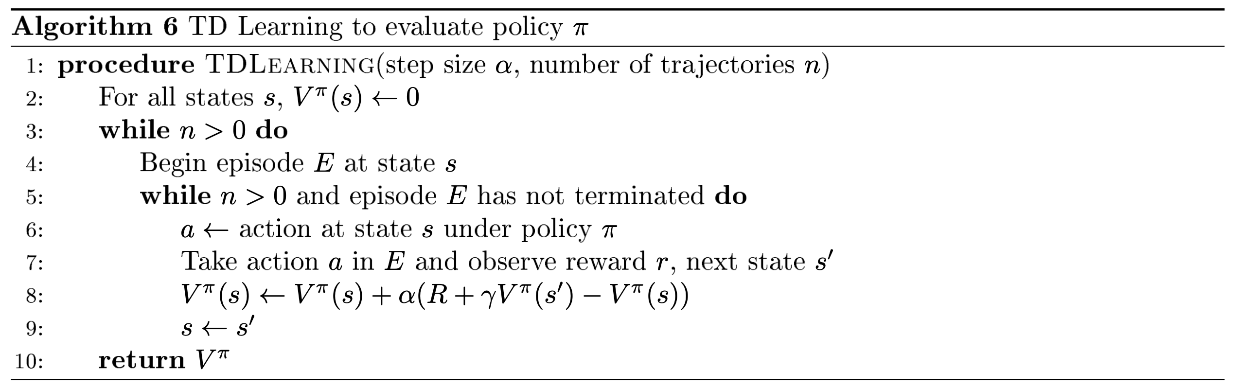
Temporal Difference (TD) learning

Combines bootstrapping (DP) and sampling (Monte Carlo).

$V^\pi(s_t)\leftarrow V^\pi(s_t) + \alpha (G_t - V^\pi(s_t))$

$= V^\pi(s_t) + \alpha (r_t + \gamma V^\pi(s_{t+1}) - V^\pi(s_t))$

We bootstrap the total returns with the next state's estimate: $r_t + \gamma V^\pi(s_{t+1})$ (called the TD target).

$\delta_t = r_t + \gamma V^\pi(s_{t+1}) - V^\pi(s_t)$ is called the TD error.

Since we don't use the total sum of discounted rewards $G_t$ we don't have to wait for the episode to finish.

• the reason why we are able to backup over one timestep in DP is because of the Markov assumption. We can use incremental Monte-Carlo with $\alpha > 1/N$ in non markovian settings.
• we proved DP converges to the true value function by proving that the Bellman backup operator is a contraction
• in TD learning, we bootstrap the next state's value to get an estimate of the current state. It is thus biased towards the next state's value.
• TD learning is also less data efficient than Monte-Carlo. Since the information only comes from next state (vs the total discounted sum of rewards of the entire episode), we neet to experience an episode $L$ times ($L$ being the length of the episode) to get the full information back to the starting state (especially impactful if high reward is experienced at the end).

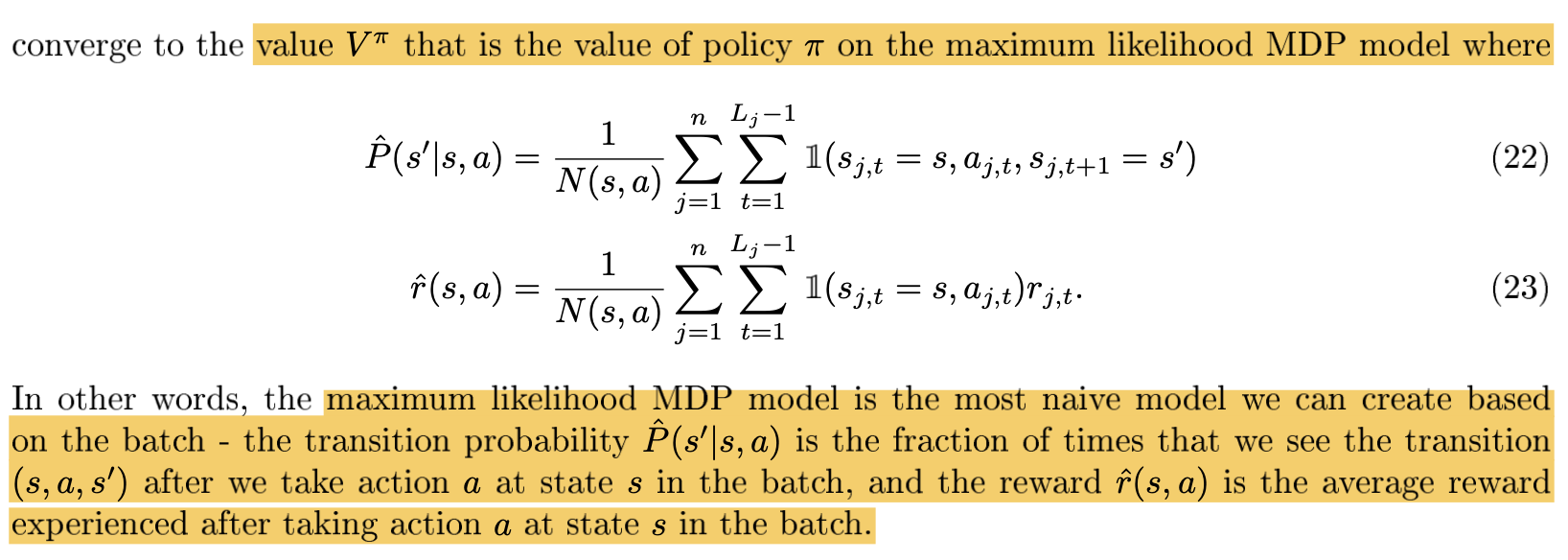
Batch Monte-Carlo and TD

• Monte-Carlo batch setting: value converges value that minimizes mean squared error (since the minimizer of $\sum (y_i - \hat y)^2$ is $\hat y = \sum y_i$)
• TD batch setting does not converge to the same value: