Assumptions

• Markov Property: $P(s_i\vert s_0,\dots, s_{i-1})=P(s_i\vert s_{i-1})$
• Finite state space: $\lvert S\rvert < \infty$
• Stationary transition probabilities (time-independent): $P(s_i=s'\vert s_{i-1}=s)=P(s_j=s'\vert s_{j-1}=s)$. We can write it as a transition probability matrix $P$ of size $\lvert S\rvert \times \lvert S \rvert$ where $P_{ij} = P(j\vert i)$.

Markov Reward Process

add:

• $R:S\to\mathbb{R}$: reward function mapping states to rewards
• $\gamma \in [0, 1]$ discount factor

Expected reward: $R(s)=\mathbb{E}[r_0\vert s_0=s]$

Stationary rewards assumption:

• $s_i=s_j\Rightarrow r_i=r_j$ (same state implies same reward)
• For stochastic rewards: $CDF(r_i\vert s_i=s)=CDF(r_j\vert s_j=s)$ and we have $R(s)=\mathbb{E}[r_0\vert s_0=s]=\mathbb{E}[r_1\vert s_1=s]=\dots$ (same state, regardless of step, implies same CDF and therefore same expected reward)

Q: A condition on the CDF implies a condition on the distribution itself

A condition on the Cumulative Distribution Function (CDF) is equivalent to a condition on the distribution itself. The CDF is a representation of the probability distribution of a random variable.

The reason the CDF might be used instead of the Probability Density Function (PDF) or Probability Mass Function (PMF) is that the CDF is defined for all kinds of random variables—discrete, continuous, and mixed—while the PDF or PMF is only defined for continuous or discrete random variables, respectively.

This condition therefore implies the condition that expected rewards be constant.

• Horizon: number of time steps in each episode (finite or infinite)
• Return: sum of discounted rewards $G_t=\sum_{i=t}^{H-1}\gamma^{i-t}r_i \forall 0\leq t \leq H-1$
• State value function: $V_t(s)=\mathbb{E}[G_t\vert s_t=s]$ (expected return starting from $s$).

Infinite horizon (with $\gamma < 1$) + stationary rewards $\Rightarrow V(s)=V_0(s)$ (stationary state value function).

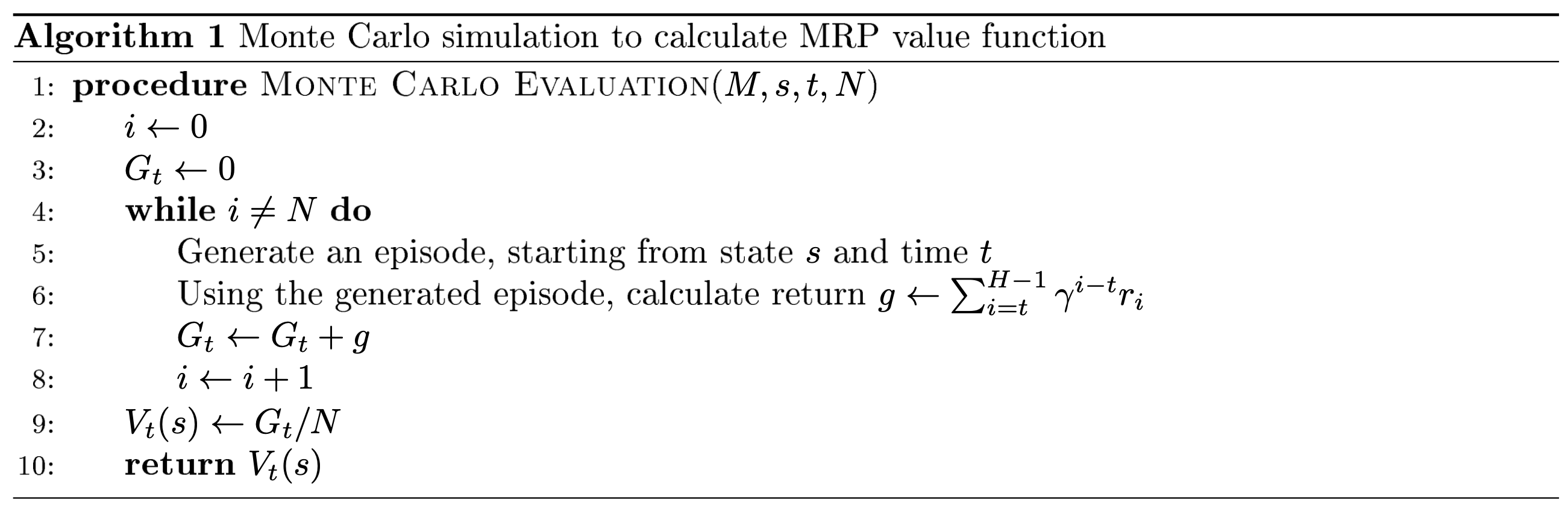
Computing the state value function

Monte Carlo Simulation

Analytic solution

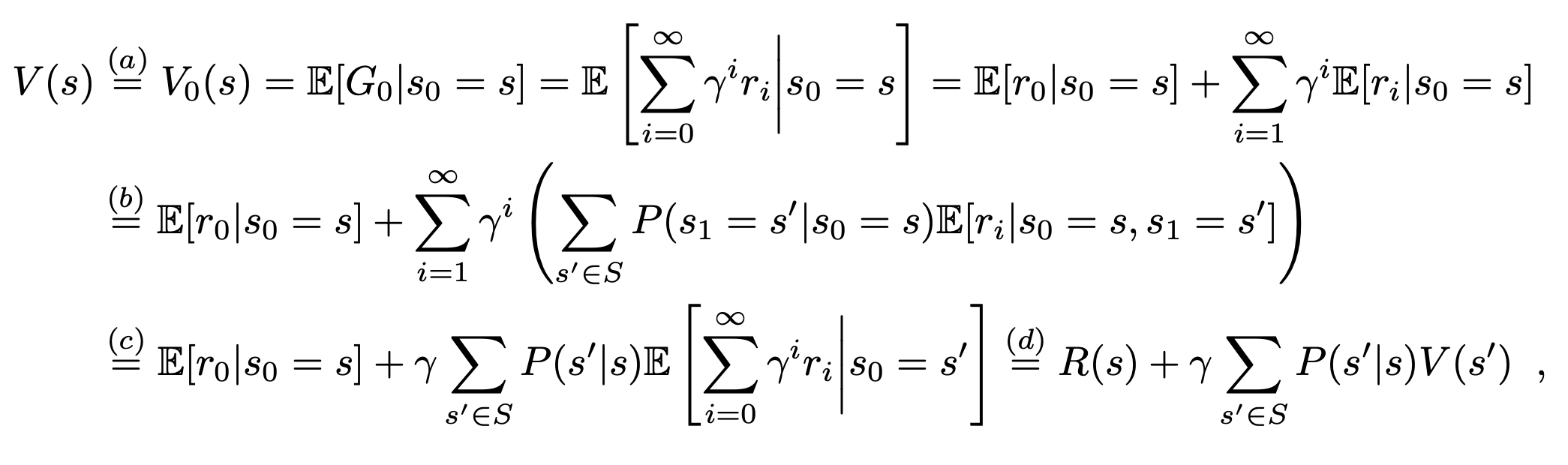
As $\lvert S\rvert < \infty$ we can write: $V=R+\gamma PV$ which has the analytical solution $V = (I-\gamma P)^{-1}R$ (complexity in $\lvert S\rvert^3$).

(this assumes that we have the transition probabilities and rewards)

Dynamic Programming solution

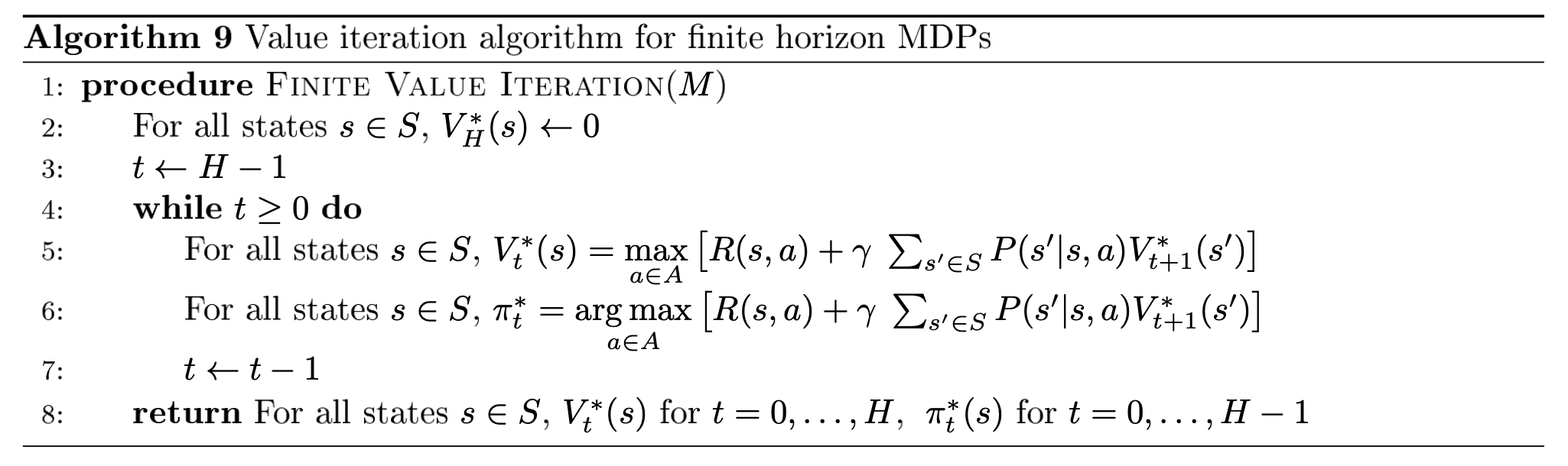
Finite horizon:

• start with $V_H(s)=0$ (by definition, there are no future steps to consider, so the expected sum of future rewards is zero)
• iterate back to $0$ with $V_t(s)=R(s)+\sum_{s'\in S}P(s'\vert s)V_{t+1}(s')$

Infinite horizon:

• we know $V$ must be time-independent
• start with two value function estimates $V'(s)\leftarrow 0 \forall s$ and $V(s)\leftarrow \infty \forall s$
• update estimate $V' = R + \gamma PV$ until $\lVert V' - V\rVert_\infty \leq \epsilon$ (infinity norm is the component with largest absolute value) and return $V'$
• see p.8 for proof of correctness

Complexity: $\lvert S\rvert^2$

Markov Decision Process

add $A$: finite set of actions available from each state $s$.

Stationary transition probabilities:

$P(s_i=s'\vert s_{i-1}=s, a_{i-1}=a)=P(s_j=s'\vert s_{j-1}, a_{j-1}=a)$ (where action precedes state)

Stationary rewards:

$R(s,a)=\mathbb{E}[r_i\vert s_i=s, a_i=a] \forall i$

Policy: probability distribution over actions given current state. Can vary with time: $\pi = (\pi_0, \pi_1, ...)$ (where subscript denotes timestep)

• State value function: $V_t^{\pi}(s)=\mathbb{E}_\pi[G_t\vert s_t=s]$. When horizon is infinite, state value function is stationary and $V^\pi(s)=V_0^{\pi}(s)$
• State action value function: $Q_t^{\pi}(s,a)=\mathbb{E}[G_t\vert s_t=s, a_t=a]$. Meaning we compute expected return given that we are in state $s$ and take action $a$. With infinite horizon: $Q^{\pi}(s,a)=Q_0^{\pi}(s,a)$

Computing state action value function for infinite horizon:

$Q^{\pi}(s,a) = R(s,a) + \gamma \sum_{s'\in S}P(s'\vert s,a)V^{\pi}(s')$

A stationary policy (i.e. $\pi=\pi_0=\pi_1=\dots$) has an equivalent markov reward process (by taking expectation over action space):

$R^{\pi}(s)=\sum_{a\in A} \pi(a\vert s)R(s,a)$

$P^{\pi}(s'\vert s)=\sum_{a\in A} \pi(a\vert s) P(s'\vert s,a)$

Can then use previous techniques to evaluate value function (we call it policy evaluation).

MDP control for infinite horizon

$\pi^*$ optimal iff $V_t^{\pi^*}(s) \geq V_t^{\pi}(s) \forall t,s$.

For infinite horizon MDP, existence of an optimal policy implies existence of a stationary optimal policy (i.e. we only need to consider stationary policies). Intuitively, if $\pi^{*} = (\pi_0^{*}, \pi_1^{*}, \dots)$ is an optimal (non-stationary) policy, we can compute $V^{\pi_i^{*}}$ which is independent of time (because horizon is infinite), for all $i$. By the definition of an optimal policy, we can just keep the $\pi_i^{*}$ that has the maximum state value function.

Moreover, there is an optimal deterministic policy $\hat\pi$ such that $V^{\hat\pi}(s) \geq V^{\pi}(s)$ for all states $s$. We can construct it from a stationary policy:

$\hat\pi(s) = \arg\max_{a\in A}\big[R(s,a) + \gamma \sum_{s'\in S}P(s'\vert s, a)V^{\pi}(s')\big], \forall s \in S$

Search for an optimal policy has been reduced to the set of deterministic stationary policies (there's $\vert A\vert^{\vert S\vert}$ possibilities).

Policy search

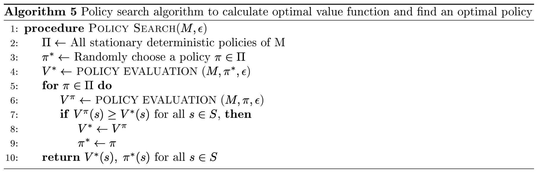
Brute force algo. Terminates because it checks all $\vert A\vert^{\vert S\vert}$ policies.

Policy iteration

more efficient.

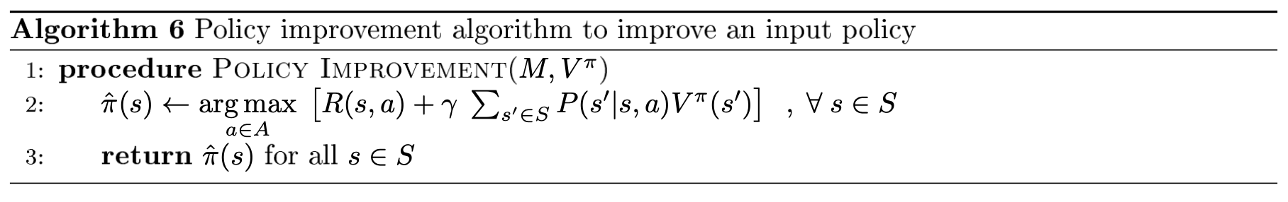
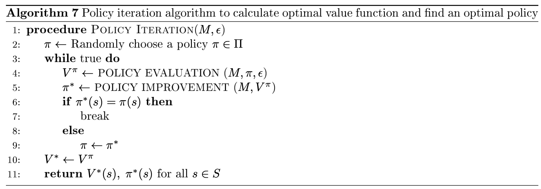
Proof of correctness: https://stats.stackexchange.com/questions/272777/policy-and-value-iteration-algorithm-convergence-conditions/299950#299950

The value functions at every iteration are non-decreasing. If we cannot improve our policy further, it means:

$\pi(s) = \arg\max_{a\in A}[R(s,a) + \gamma \sum_{s' \in S} P(s'\vert s,a)V^{\pi}(s')], \forall s\in S$

thus:

$V^{\pi}(s) = \max_{a\in A}[R(s,a) + \gamma \sum_{s'\in S}P(s'\vert s, a)V^{\pi}(s')$

which is the Bellman optimality equation.

Value iteration

We look for a fixed value function instead of a fixed policy.

MDP control for finite horizon

In the finite horizon state, there's an optimal deterministic policy but it is no longer stationary (at each time $t$, the policy is different).