OpenAI, March 2022

with info from https://huggingface.co/blog/rlhf

Highlights

• fine-tune GPT-3 using supervised learning. Collect dataset of rankings of model outputs. Fine-tune using reinforcement learning from human feedback.
• 1.3B parameters InstructGPT preferred over 175B GPT-3
• alignment to user's intent.

Intro

Next token prediction objective $\neq$ "follow user's instructions helpfully and safely"

To compensate for the loss, we use metrics like BLEU or ROUGE that try to compare generate text to human text with simple ngrams.

Explicit intentions: following instructions

Implicit intentions: staying truthful, not being biased, toxic, harmful

1. Supervised fine-tuning (optional)

Team of 40 screened contractors to label data. Collect human written demonstrations of desired output behavior on prompts submitted to OpenAI API and some labeler-written prompts. Train supervised learning baselines.

• train for 16 epochs using cosine learning rate decay and residual dropout of 0.2
• they found that model overfits on validation loss after 1 epoch but training for longer improves reward modeling score and human preference.

residual dropout:

• with probability $p=0.2$, set activation to 0. This will mean this neuron is ignored during backprop.
• with probability $1-p$, normalize activation $h := h/(1-p)$

cosine learning rate decay (with restart):

Anthropic used transformer models from 10 million to 52 billion params.

DeepMind used their 280 billion param model Gopher.

2. Reward modeling

Starting from supervised fine-tuned model, remove the softmax layer (they call it unembedding layer) and output a scalar reward instead (scalar reward represents human preference). Model size: 6B instead of 175B (unstable training).

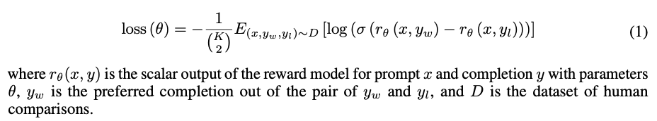
Trained on a dataset of comparisons between two model outputs. Use a cross-entropy loss: the difference in rewards represents the log odds that one response will be preferred to the other by a human labeler.

Collect dataset of human-labeled comparisons between outputs from models on a larger set of API prompts. Train a reward model on this dataset to predict which model output labelers would prefer.

Q: why not ask the humans to score the model output with a scalar instead?

A: Different humans assign different scores based on their values, meaning scores are uncalibrated and noisy. Rankings are more robust.

Elo system (like in chess) is then used to generate a scalar reward signal for training.

Comparisons are very correlated within each labeling task. when simply shuffling all comparisons into one dataset, a single pass over the dataset causes reward model to overfit. (if each of $2$ in $K$ comparisons is treated as separate data point, each completion will be repeated multiple times in the dataset, causing overfitting). Instead, all $2$ among $K$ comparisons for each prompt is a single batch element. More efficient because it requires a single forward pass for each completion instead of $2$ among $K$ forward passes for $K$ completions. It no longer overfts. Q: unclear? are they outputting a vector instead of a scalar?

Loss function for reward model:

Intuitively, reward model should have similar capacity as the text generation model to understand the text given to them.

3. Reinforcement learning

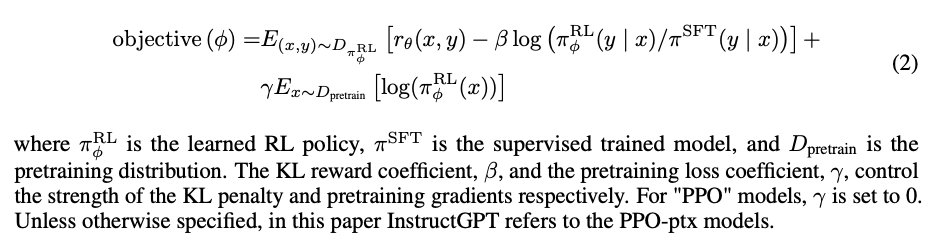
Use this reward model as a reward function and fine-tune the supervised learning baseline to maximize this reward using PPO algorithm. Parameters of the LM are frozen.

Formulating as a RL problem:

• policy: language model that takes in a prompt and returns a sequence of text (until a <EOS> token is generated)
• action space: all tokens in vocabulary (50k tokens)
• observation space: distribution of possible input token sequences (dimension = vocab size ^ input length)
• reward function: combination of preference model + constraint on policy shift (KL penalty, see below). The reward model ingests the whole sequence and outputs a single scalar.

For every token generated in the sequence, the model calculates the gradient of the reward with respect to the parameters. The reward function (based on human feedback or a learned model) is non-differentiable, so techniques like the policy gradient theorem are applied, which rely on sampling complete sequences.

The KL penalty is applied to each token generated auto-regressively: at each token compare the logits of the fine-tuned model to that of the base model.

The reward function is non-differentiable because:

• It’s not computed as a continuous function of the model’s internal parameters (it’s often just a score or label based on external evaluation).
• It operates on the entire output sequence, which is generated via sampling or decoding, introducing discontinuities.

Because the reward function doesn’t provide gradients directly, we can’t back-propagate through it in the conventional sense.

Bandit environment, presents a random customer prompt and expects a response to the prompt. Given the prompt and response, it produces a reward determined by the reward model and ends the episode.

Add a per-token KL penalty from the supervised fine-tuned model at each token to mitigate over-optimization of the reward model. Penalizes RL policy from moving substantially away from initial pre-trained model. Without it, model could output gibberish that fools the reward model into giving it a high reward.

RL objective:

Evaluation: labelers rate quality of model outputs on test set consisting of prompts from held-out customers (not represented in training data).

Appendix: the policy-gradient theorem

The policy gradient theorem is a foundational concept in reinforcement learning (RL) that allows optimization of policies even when the reward function is non-differentiable. It works by estimating gradients indirectly using sampling.

For language models:

• Policy: The probability distribution $\pi_\theta(a \vert s)$ , where $a$ is a token or sequence of tokens (action), $s$  is the prompt (state), and  $\theta$  represents the model’s parameters.
• Goal: Maximize the expected reward $\mathbb{E}[R]$, where $R$  is the reward for a sequence.

The policy gradient theorem states:

In practice, it's estimated using Monte-Carlo sampling.

This is derived by introducing the logarithmic trick into $\nabla_\theta J(\theta) = \nabla_\theta \mathbb{E}{\pi\theta}[R]$:

This equation provides a way to estimate the gradient of the expected reward with respect to the model parameters $\theta$ , using the log probabilities of actions (sequences) weighted by the reward $R$.

Dealing with the log probabilities is easier because, the normalization term in the softmax cancels out and the product of probabilities turns into a sum (which is easier to differentiate than a product).

Steps:

1. Sampling: Generate a sequence  $a \sim \pi_\theta(a \vert s)$  from the model.

2. Reward Evaluation: Compute  $R$  for the generated sequence using the reward model or human feedback.

3. Gradient Estimation: Use the sampled sequence to compute:

Here,  $\nabla_\theta \log \pi_\theta(a \vert s)$ represents the gradient of the log-probability of the sampled sequence, which is differentiable.

Since the output sequence is generated in an auto-regressive manner, the log proba of the sequence is the sum of the log probabilities of each incremental token and: