source

Two kinds of recommendations:

• home page recommendations: personalized to a user based on their interests
• related item recommendations

Common architecture:

1. candidate generation (reduce corpus: billions to a few 100k)

2. scoring (reduce corpus: few 100k to 10, system can use more complex model)

3. re-ranking: additional constraints (e.g. items that the user explicitly disliked / boost the score of fresher content)

Candidate generation

• Content-based filtering: use similarity between items

• Collaborative filtering: similarities between queries (users) and items

• Similarity metrics:

  • dot product

  • cosine similarity = dot product of normalized vectors

  • euclidean distance = $\lVert q-x\rVert = \sqrt{\sum_i (q_i - x_i)^2}$. When $q$ and $x$ are normalized, $q$, $x$ and $q-x$ are the sides of an equilateral triangle with lenght 1. Therefore:

  $1/2\lVert q-x\rVert^2 = 1/2(q^Tq - 2q^Tx + x^Tx) = 1/2(1 - 2cos(q,x)+1)=1-cos(q,x)$

• Items that appear frequently in the dataset have embeddings with larger norms. If capturing popularity is desirable, you can use dot product. In practice, you can define a variant that puts less emphasis on the norm: $\lVert q\rVert^\alpha \lVert x\rVert^\alpha \cos(q,x), \alpha \in (0,1)$

• Initialization: if embeddings are initialized with a large norm, rare items (which are less frequently updated) will have a larger norms.

Content-based filtering

• recommendations specific to a single user
• $q$ (user) and $x$ (item) share the same feature space
• evaluate the similarity between $q$ and $x$ (e.g. dot product)
• model can only make recommendations based on existing interests of the user. In other words, the model has limited ability to expand on the users' existing interests.
• features are hand-engineered. I.e. they're not embeddings.

Collaborative filtering

• recommendations based both on similar users and similar items to its history (recommendations are thus more serendipitous, users can discover new interests)
• embeddings can be learned automatically, without relying on hand-engineering of features
• feedback matrix where rows = users and columns = items
• explicit feedback (likes, ratings) vs implicit feedback (watch time)

Matrix factorization

Simple embedding model.

Given feedback matrix $A\in \mathbb{R}^{m\times n}$ where $m$ is the number of users and $n$ the number of items:

• learn user embedding matrix $U\in \mathbb{R}^{m\times d}$ where $d$ is embedding dimension
• learn item embedding matrix $V\in \mathbb{R}^{n\times d}$

Such that: $A\approx UV^T$

• $A$ is very sparse

Objective functions

• Naive least squares over observed entries: $\sum_{(i,j)\in \text{obs}}(A_ij - <U_i,V_j>)$. If we only sum over observed entries, a matrix of all $1/\sqrt(d)$ for $U$ and $V$ produces minimal loss. The model does not learn how to place the embeddings of irrelevant movies. This is known as folding.
• Treat unseen entries as zero and minimize Frobenius norm: $\lVert A - UV^T\rVert_F^2$. Solvable using singular value decomposition. However, since $A$ is sparse, the solution $UV^T$ will likely be close to zero.
• weighted MSE: $\sum_{(i,j)\in\text{obs}} w_ij(A_{ij}-<U_i,V_j>)^2 + w_0$
• • $l_2$ regularization: $\frac{1}{n}\sum_i \lVert U_i\rVert^2 + \frac{1}{m}\sum_j \lVert V_j \rVert^2$
• • gravity, a global prior that pushes the prediction of any pair towards zero: $\frac{1}{nm}\sum_{(i,j)\notin \text{obs}} <U_i, V_j>^2$
• balance the two regularization terms with hyper-parameters

Folding

• Some categories of queries and items (such as language of a user / video on YouTube) may only interact among each other.
• model learns how to place the query/item embeddings within a category but embeddings from different colors may end up in the same region of the embedding space by chance.
• This phenomenon is known as folding and can lead to spurious recommendations (model predicts a high score for an item from a different group)

Illustration of the folding phenomenon: squares = entities, circles = items, colors = categories

Optimizer

• Stochastic Gradient Descent (generic)
• Weighted Alternating Least Squares: specialized for this objective
• Objective is convex in $U$ and $V$ but not jointly convex
• WALS alternates between fixing $U$ and solving for $V$ and vice-versa until convergence
• WALS converges faster than SGD

Cold start problem

• Given new item $i_0$ that has a few interactions with users, we can generate its embedding by keeping $U$ fixed and performing one iteration of WALS over $v_{i_0}$
• heuristics-based: average embeddings of items from the same category

Including side features for query/item

Define block matrix:

$\bar{A} = \begin{pmatrix}A & F_i\\F_u & \vec{0}\end{pmatrix}$

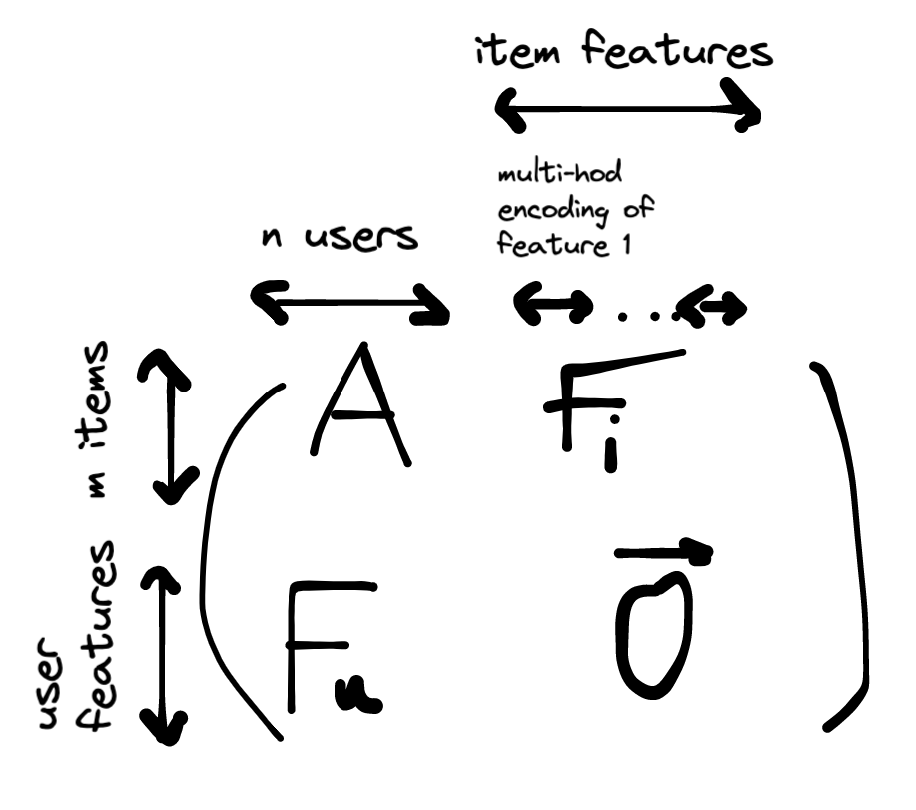
Where $F_u$ is the user features matrix and $F_i$ is the item features matrix.

Since $A$ is sparse, we can use tf.SparseTensor(indices, values, dense_shape) for efficient representation (only store the non-zero entries).

Initialization. Let the ratings vector $X = \sigma Z$ where each entry of $Z$ follows a standard normal distribution. We have that $X \sim \mathcal{N}(0, \sigma^2)$.

$\lVert X\rVert^2 = \sum \sigma^2 Z_i^2 \sim \sigma^2\chi^2(n)$. Expected norm: $\mathbb{E} \lVert X\rVert^2 = \sigma^2 \mathbb{E}[\chi^2(n)] = n \sigma^2$. Therefore we should init each embedding vector with $\mathbb{E} \lVert X\rVert = \sigma \sqrt{n}$.

Deep neural networks

Multiclass prediction problem using softmax model:

• input is user query:

  • dense features: watch time, time since last watch

  • sparse features: watch history, country

• output is probability vector over corpus of items, representing the probability of interacting with the item (e.g. click or watch probability)

Architecture

• input layer -> hidden layers with ReLU activations -> softmax layer
• $\hat p = \text{softmax}(\underbrace{f(x)}_{\in\mathbb{R}^d}\underbrace{W^T}_{\in\mathbb{R}^{d,\lvert items\rvert}})$ where $W$ is the learned item embedding matrix and $f(x)$ the output of the neural net, the embedding of the query.
• The softmax outputs a probability distribution over the dot product (similarity) of the item embeddings and the query embedding.
• Loss: cross-entropy loss between predicted probability distribution and ground truth (items the user has interacted with, as a normalized multi-hot distribution)
• computing the gradient on the entire corpus is prohibitively expensive. If we only train on positive pairs however, the model suffers from folding. We use negative sampling to include items that are irrelevant to the query in the loss.
• if we sample uniformly, some negatives might not contribute enough to the gradient (they are too obvious). Hard negatives: we can assign a higher probability to items $j$ with a higher score $<f(x),V_j>$ (they are harder to differentiate from the true positives).

How to include item features

Use two-tower neural net:

* one NN maps query featuers to query embedding

* one NN maps item features to item embedding

* output is the dot product of the two

Matrix factorization vs deep neural networks

• matrix factorization is better for large corpora: easier to scale, cheaper to query (query embedding does not need to be computed at query time, it's only a look up in the user embeddings matrix), less prone to folding (by adjusting unobserved weight in WALS)
• DNN models can better capture personalized preferences. They are preferable for scoring because they can use more feature and are more expressive. It is usually acceptable for DNN models to fold since you mostly care about ranking a prefiltered set of candidates assumed to be relevant.

Retrieval

• This is a nearest neighbors problem. Return top $k$ items according to similarity score.

• For large-scale retrieval, you can:

  • precompute the scores offline

  • use approximate nearest neighbors

Scoring

• Recommendation system may have multiple candidate generation models

• model combines candidates, scores them and ranks them accordingly

• why not let the candidate generator score?

  • scores of different candidate generation models might not be comparable

  • with a smaller pool of candidates, scoring model can afford to use more features and parameters and thus better capture context

• objective functions:

  • maximize click rate: system recommends click-bait. Poor user experience and user's interest may quickly fade.

  • maximize watch time: system recommends very long videos. Poor user experience. Multiple short watches can be just as good as one long watch.

  • increase diversity and maximize session watch time: recommend shorter videos, but ones that are more likely to increase engagement.

• positional bias: items that appear lower on the screen are less likely to be clicked.

Re-ranking

• freshness:

  • re-run training (warm start) as often as possible

  • new users: average a cluster of embeddings based on user features or use a neural net that takes user features as input

  • add document age as a feature

• diversity (lack of diversity causes boring user experience):

  • train multiple candidate generators using different sources

  • train multiple rankers using different objective functions

  • re-rank items based on genre or metadata

• fairness:

  • track metrics for each demographics to watch for biases

  • make separate models for underserved groups