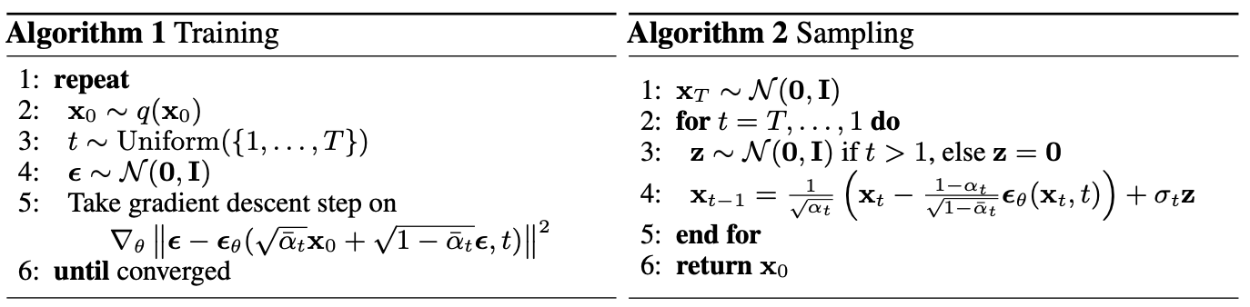
Parameterized Markov chain trained using variational inference to produce samples matching the data after finite time. Transitions of this chain are learned to reverse a diffusion process, which is a Markov chain that gradually adds noise to the data in the opposite direction of sampling until signal is destroyed.

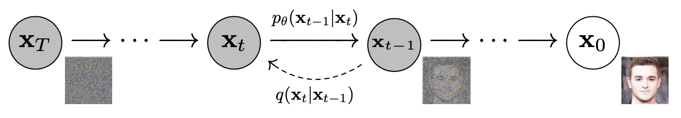
Let $p_\theta$ be the parameterized reverse process. It's defined as Markov chain with learned Gaussian transitions starting at $p(x_T)=\mathcal{N}(x_T; 0, I)$.

$p_\theta(x_{0:T}) := p(x_T)\prod_{t=1}^T p_\theta(x_{t-1}\vert x_t)$

$p_\theta(x_{t-1}\vert x_t):= \mathcal{N}(x_{t-1};\mu_\theta(x_t, t), \Sigma_\theta(x_t, t))$

The forward process or diffusion process $q(x_{1:T}\vert x_0)$ is fixed to a Markov chain that gradually adds Gaussian noise to the data according to a variance schedule $\beta_1,\dots,\beta_T$:

$q(x_{1:T}\vert x_0):= \prod_{t=1}^T q(x_t\vert x_{t-1})$

$q(x_t\vert x_{t-1}) := \mathcal{N}(x_t;\sqrt{1-\beta_t}x_{t-1}, \beta_t I)$

In practice $\beta_i$'s are linearly increasing constants. Therefore, the forward process has no learnable parameter.

Evidence lower bound

Goal is to maximize log-likelihood of original image under reverse process: $\log p_\theta(x_0)$.

$p_\theta (x_0\vert x_{1:T})p(x_{1:T})d(x_{1:T})$

Let's refer to $x_{1:T}$ as latent variable $z$.

We can use importance sampling to estimate the log likelihood:

$p_\theta (x_0) = \mathbb{E}_{z\sim q(z\vert x_0)}[\frac{p_\theta(x_{0:T})}{q(x_{1:T}\vert x_0)}]$

By Jensen's inequality:

$\log p_\theta(x_0) = \log \mathbb{E}_q[\frac{p_\theta(x_{0:T})}{q(z\vert x_0)}] \geq \mathbb{E}[\log \frac{p_\theta(x_{0:T})}{q(x_{1:T}\vert x_0)}]$

(multiplying my $-1$ and inverting the ineq. yields eq. 3 of the paper):

Paper then rewrites it as:

$L_T$ can be ignored since the forward process has no learnable parameters.

$L_{t-1}$ can be rewritten as:

To obtain discrete log-likelihoods, the last term of the reverse process is set to an independent discrete decoder:

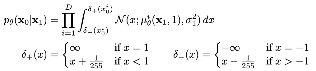
where $D$ is the data dimensionality. The reason is, since pixels are discrete and exact values are a zero probability event in continuous distributions, we integrate around the pixel's region (between $x-1/255$ and $x+1/255$).

At the end of sampling, we display $\mu_\theta(x_1, 1)$ noiselessly.

Q: "the variational bound is a lossless codelength (log-likelihood) of discrete data, without need of adding noise to the data or incorporating the Jacobian of the scaling operation into the log likelihood."

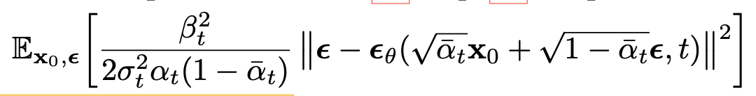
They found it beneficial to sample quality to discard the weighting term in the training objective. This down-weights loss terms corresponding to small $t$ (too easy to learn).

Experiment

Architecture

• Backbone of PixelCNN++ which is a U-Net based on a Wide ResNet ???
• replaced weight normalization with group normalization to make implementation simpler
• $32x32$ models use 4 feature map resolutions ($32x32$ to $4x4$) and $256x256$ models use 6.
• two convolutional residual blocks per resolution level and self-attention blocks at the $16x16$ resolution between the convolutional blocks.
• Parameters are shared accross time steps and diffusion time $t$ is specified by adding the Transformer sinusoidal position embedding into each residual block.
• CIFAR10 model has 35.7 million params. LSUN and CelebA-HQ models have 114 million params.

Training

We used TPU v3-8 (similar to 8 V100 GPUs) for all experiments. Our CIFAR model trains at 21 steps per second at batch size 128 (10.6 hours to train to completion at 800k steps), and sampling a batch of 256 images takes 17 seconds. Our CelebA-HQ/LSUN (2562) models train at 2.2 steps per second at batch size 64, and sampling a batch of 128 images takes 300 seconds. We trained on CelebA-HQ for 0.5M steps, LSUN Bedroom for 2.4M steps, LSUN Cat for 1.8M steps, and LSUN Church for 1.2M steps. The larger LSUN Bedroom model was trained for 1.15M steps.

Hyperparameters

• $T=1000$. $\beta_1=10^{-4}$ increasing linearly to $\beta_T=0.02$ (such that $L_T\approx=0$).
• We set the dropout rate on CIFAR10 to 0.1 by sweeping over the values $\{0.1, 0.2, 0.3, 0.4\}$. Without dropout on CIFAR10, we obtained poorer samples reminiscent of the overfitting artifacts in an unregularized PixelCNN++
• We used random horizontal flips during training for CIFAR10; we tried training both with and without flips, and found flips to improve sample quality slightly. We also used random horizontal flips for all other datasets except LSUN Bedroom.
• We tried Adam and RMSProp early on in our experimentation process and chose the former. We left the hyperparameters to their standard values. We set the learning rate to 2 × 10−4 without any sweeping, and we lowered it to 2 × 10−5 for the 256 × 256 images, which seemed unstable to train with the larger learning rate.
• We set the batch size to 128 for CIFAR10 and 64 for larger images. We did not sweep over these values.
• We used exponential moving average on model parameters with a decay factor of 0.9999

Sample quality

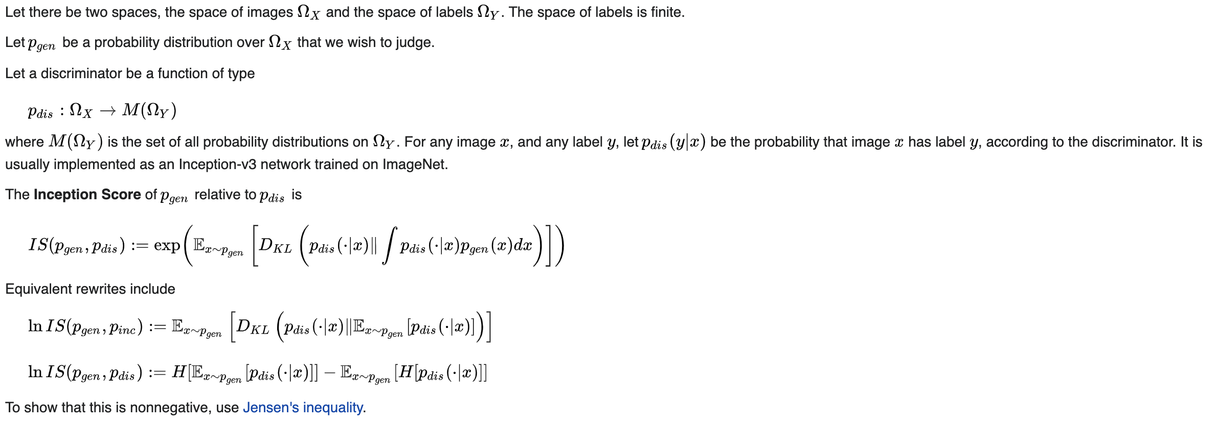
Inception score

wikipedia

Used to assess the quality of images created by a generative image model. The score is calculated based on the output of a separate, pretrained Inceptionv3 image classification model applied to a sample of (typically around 30,000) images generated by the generative model. The Inception Score is maximized when the following conditions are true:

1. The entropy of the distribution of labels predicted by the Inceptionv3 model for the generated images is minimized. In other words, the classification model confidently predicts a single label for each image. Intuitively, this corresponds to the desideratum of generated images being "sharp" or "distinct".

2. The predictions of the classification model are evenly distributed across all possible labels. This corresponds to the desideratum that the output of the generative model is "diverse"

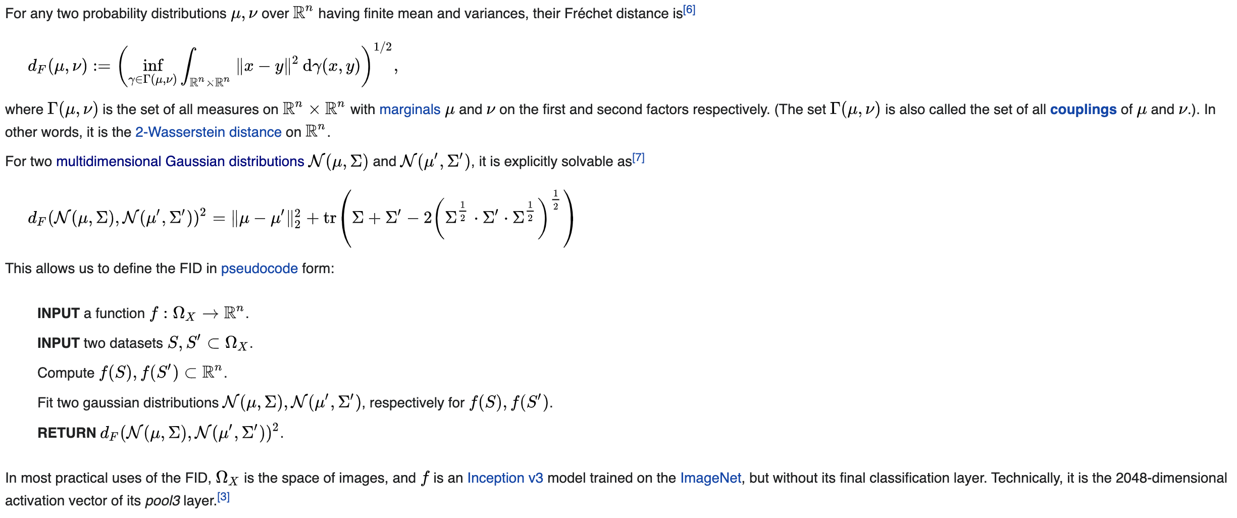
Fréchet Inception Distance (FID score)

wikipedia

Unlike the earlier inception score, which evaluates only the distribution of generated images, the FID compares the distribution of generated images with the distribution of a set of real images ("ground truth").

The FID metric was introduced in 2017, and is the current standard metric for assessing the quality of generative models as of 2020. It has been used to measure the quality of many recent models including the high-resolution StyleGAN1 and StyleGAN2 networks.

Rather than directly comparing images pixel by pixel (for example, as done by the L2 norm), the FID compares the mean and standard deviation of the deepest layer in Inception v3. These layers are closer to output nodes that correspond to real-world objects such as a specific breed of dog or an airplane, and further from the shallow layers near the input image. As a result, they tend to mimic human perception of similarity in images

Negative log-likelihood (= lossless codelength)