source

Overview

• Collaborative filtering:

  • memory-based: e.g. item-based or user-based using nearest neighbor (limitations in dealing with sparse and large-scale data since it computes similarity scores)

  • model-based: e.g. latent factor models such as matrix factorization or neural networks

• Implicit and explicit feedback

• recommendation tasks:

  • rating prediction

  • top-$n$ recommendation (item ranking)

  • sequence-aware recommendation

  • click-through rate prediction: $CTR=\frac{\#\text{Clicks}}{\#\text{Impressions}}$. Usually a binary classification problem (click or no click).

  • cold-start recommendation

Matrix factorization

Factorize the user-item interaction matrix (e.g. rating matrix) into a product of two lower-rank matrices, capturing the low-rank structure of the user-item interactions.

See this paragraph for details.

Evaluation metric: root mean squared error between observed and predicted interactions.

AutoRec: rating prediction with autoencoders

• Matrix factorization is a linear model and thus does not capture nonlinear relationships
• AutoRec differs from a traditional autoencoder in that, rather than learning the latent representations, it focuses on reconstructing the output layer.
• it uses a partially observed interaction matrix as input, aiming to reconstruct a completed rating matrix.
• Two variants: user-based and item-based

Item-based AutoRec

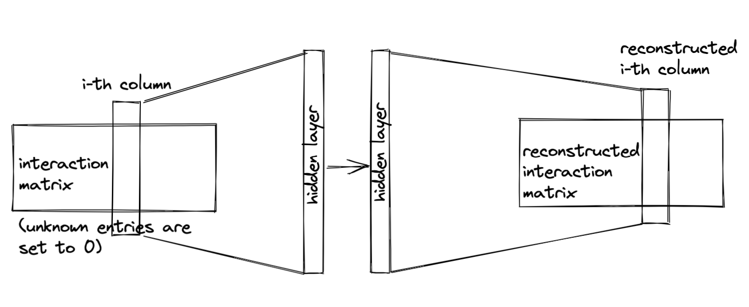
Reconstruction error: $\arg\min_{\underbrace{W,V}_{\text{weights}},\underbrace{\mu,b}_{\text{biases}}} \sum_{i \in\text{columns of } R} \lVert R_i - h(R_i)\rVert_\text{observed entries}^2 + \lambda(\lVert W\rVert_F^2 + \lVert V\rVert_F^2)$ where $R$ is the ratings matrix

Personalized Ranking for Recommender Systems

• former methods only use explicit feedback (expensive to collect and most signals lie in implicit feedback)
• ratings might not be missing at random but because of users' preferences

Three types of ranking losses:

• pointwise approach: consider a single interaction at a time (e.g. matrix factorization and AutoRec are optimized with pointwise objectives)
• pairwise approach: consider a pair of items for each user and aim to approximate the optimal ordering for that pair. More suitable for ranking task. (see next sections: Bayesian Personalized Ranking loss and Hinge loss)
• Listwise approach: approximate the ordering of the entire list of items (e.g. direct optimizing the ranking measures such as normalized discounted cumulative gain). More complex and compute-intensive

Bayesian Personalized Ranking Loss

See original paper Bpr: bayesian personalized ranking from implicit feedback

Training data: tuples $(u, i, j)$ which represents that the user $u$ prefers item $i$ over item $j$ (both positive and negative pairs i.e. missing values, assumes user prefers positive item over all other non-observed items).

BPR aims to maximize the posterior probability of model parameters given desired personalized ranking for user $u$: $p(\Theta \vert \text{ranking}_u)$

$\begin{aligned} \ln p(\Theta\vert \text{ranking}_u) & \propto \ln p(\text{ranking}_u\vert \Theta)p(\Theta) \\& = \ln \prod_{(u,i,k)}\underbrace{\sigma}_{\text{sigmoid function}}(\hat y_{ui} - \hat y_{uj})p(\Theta) \\& = \sum_{(u,i,j)} \ln \sigma(\hat y_{ui} - \hat y_{uj}) + \ln \underbrace{p(\Theta)}_{\sim \mathcal{N}(0, \lambda_\Theta I)} \\& = \sum_{(u,i,j)} \sigma(\hat y_{ui} - \hat y_{uj}) - \lambda_\Theta \lVert \Theta\rVert^2\end{aligned}$

Where $i$ is taken from the positive items and $j$ is taken from the negative items for user $u$. $\hat y_{ui}$ is the predicted score of user $u$ to item $i$.

Hinge Loss

Often used in Support Vector Machine classifiers.

$\sum_{(u,i,j)} \max(m-\hat y_{ui} + \hat y_{uj}, 0)$

where $m$ is the safety margin. It aims to push negative items away from positive items.

Neural Collaborative Filtering for Personalized Ranking

• implicit feedback (clicks, buys, watches)

NeuMF

• NeuMF (for neural matrix factorization, He et al, 2017) leverages non-linearity of neural nets to replace dot products in matrix factorization
• unlike the rating prediction task in [AutoRec](d2l_recommender_systems_course#AutoRec rating prediction with autoencoders), the model generates a ranked recommendation list to each user based on the implicit feedback
• fuses two subnetworks: generalized matrix factorization (GMF) and multi-layer perceptron (MLP)
• trained using pairwise ranking loss. Thus important to include negative sampling.

Generalized matrix factorization (GMF)

$\begin{aligned}x & = p_u \cdot q_i \\\hat y_{u,i} & = \sigma(h^T x)\end{aligned}$

• $p_u$ is the $u$-th row of $P \in \mathbb{R}^{m\times k}$ (the user embeddings)
• $q_i$ is the $i$-th row of $Q \in \mathbb{R}^{n\times k}$ (the item embeddings)
• $m$ is the number of users
• $n$ is the number of items
• $k$ is the number of latent dimensions

Multi-layer perceptron

• uses concatenation of user and item embeddings as input $[u_u, v_i]$ (not the same ones as the GMF layer) and passes it through a multi-layer perceptron

Final layer

$\hat y_{u,i}$ is the prediction score of user $u$ for item $i$:

$\hat y_{u,i} = \sigma(h^T[\text{GMF}(p_u, q_i), \text{MLP}([u_i, v_i])$

Evaluation

Split dataset by time into training and test sets.

Hit rate at given cut-off (Hit @ r)

$\text{Hit @ r} = \frac{1}{\text{user set}}\sum_{u\in \text{user set}} \mathbb{I}(\text{rank}_{u, g_u} \leq r)$

Where $\text{rank}_{u, g_u}$ denotes the ranking of ground truth item $g_u$ of the user $u$ (the one that the user clicked on) in the predicted recommendation list (ideal ranking is 1).

Area under curve (AUC)

Proportion of times where the predicted rank of the ground truth item was better than that of irrelevant items.

$\text{AUC}=\frac{1}{\text{user set}}\sum_{u\in\text{user set}} \frac{1}{\lvert \mathcal{D}\rvert}\sum_{j\in \mathcal{D}} \mathbb{I}(\text{rank}_{u, g_u} < \text{rank}_{u, j})$

Where $\mathcal{D} = \text{item set} - \text{candidate items of user u}$

Sequence-Aware Recommender Systems

• in previous sections, we abstract the recommendation task as a matrix completion problem without considering users' short-term behaviors
• take sequentially-ordered user interaction logs into account
• modeling users' temporal behavioral patterns and discovering their interest drift
• point-level pattern: indicates impact of single item in historical sequence on target item
• union-level pattern: implies influences of several previous actions on subsequent target

CASER

Convolutional Sequence Embedding Recommendation

Let sequence $(\underbrace{S_1^u}_{\text{first item}}, S_2^u \dots, )=S^{u}$ denote the ordered sequence of items for user $u$.

Suppose we take previous $L$ items into consideration. Embedding matrix that represents former interactions for time step $t$ can be contstructed: $E^{(u, t)} = [q_{S_{t-L}^{u}}, \dots, q_{S_{t-1}^{u}}]^T \in \mathbb{R}^{L\times k}$ where $q_i$ is the $i$-th row of item embeddings $Q\in\mathbb{R}^{n\times k}$.

$E^{(u, t)}$ can be used to infer the transient interest of user $u$ at time-step $t$ and is used as input to the subsequent components.

$E^{(u, t)}$ is passed through an horizontal convolutional layer and a vertical convolutional layer in parallel. Their outputs are concatenated and passed into a fully-connected layer to get the final representation.

$\begin{aligned}o & = \text{HConv}(E^{(u, t)}, \text{horizontal filters})\\o' & = \text{VConv}(E^{(u, t)}, \text{vertical filters})\\z & = \sigma(W[o,o']^T + b)\\\hat y_{u,i,t} & = v_i [z, p_u]^T + b_i \\\end{aligned}$

Where $V$ is another item embedding matrix, $P$ is the user embedding matrix for user's general tastes.

Model can be learned with BPR or Hinge loss.

Data generation process:

See also Session-based recommendations with RNNs

Feature-rich recommender systems

In addition to interaction data (sparse and noisy), integrate features of items, profiles of users and in which context the interaction occured.

Factorization Machines

• supervised algo used for classification, regression and ranking tasks
• generalization of linear regression and matrix factorization
• reminiscent of support vector machines with polynomial kernel
• can model $\chi$-way variable interactions ($\chi$ is polynoimal order, usually 2), fast optimization algo reduces polynomial computation time to linear complexity

2-way factorization machines

Let $x\in\mathbb{R}^d$ denote feature vectors of one sample, $y$ corresponding label (either real-valued label or class label). 2-way factorization machine defined as:

$\hat{y}(x) = w_0 + \sum_{i=1}^d w_i x_i + \sum_{i=1}^{d}\sum_{j=i+1}^{d}\underbrace{<v_i, v_j>}_{\text{interaction between i-th and j-th feature}}x_i x_j$

where $w_0\in\mathbb{R}$ is the global bias; $w\in\mathbb{R}^d$ denotes weights of $i$-th variable; $V\in\mathbb{R}^{d\times k}$ represents feature embeddings ($k$ being dimensionality of latent factors)

First two terms correspond to linear regression and last term is an extension of matrix factorization.

Efficient optimization criterion

Naive evaluation leads to $\mathcal{O}(kd^2)$

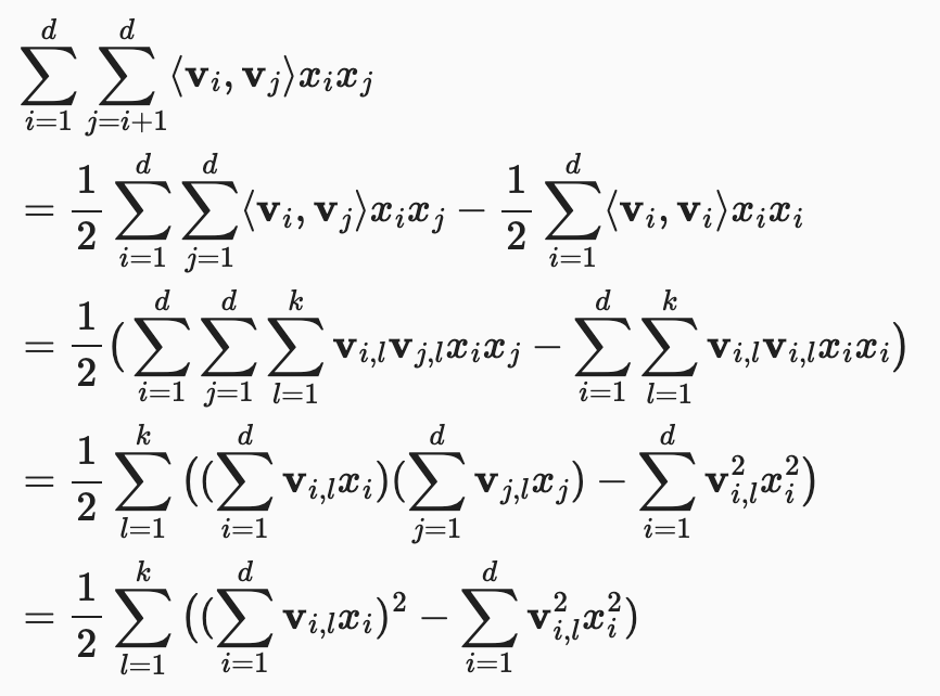
First line: total sum is twice the triangular sum - sum of diagonal.

Time complexity becomes linear: $\mathcal{O}(kd)$. Moreover, only non-zero elements need to be computed (efficient for sparse features).

Loss functions: MSE for regression, cross-entropy for classification, BPR loss for ranking.

Deep Factorization Machines

Factorization machines still combines interactions in a linear model. Higher order feature interactions (> 2) usually lead to numerical instability and high computational complexity.

Deep neural networks can learn sophisticated (nonlinear + higher order) feature interactions with rich feature representations.

DeepFM (Guo et al., 2017) has two components: factorization machine and multi-layer perceptron.

FM component's output is: $\hat{y}^{(FM)}$ (see previous section)

MLP component:

Let $e_i\in\mathbb{R}^k$ be the latent feature vector of feature $i$.

$\begin{aligned}z^{(0)} & = [e_1,\dots,e_f] \\z^{(l)} & = \text{activation}(W^{(l)}z^{(l-1)} + b^{(l)})\end{aligned}$

Output is $\hat{y}^{(MLP)}$

Both outputs are combined in sigmoid function: $\hat{y} = \sigma(\hat{y}^{(FM)} + \hat{y}^{(MLP)})$.

See also Neural factorization machines for sparse predictive analytics