Adjustment for direct causes (p.65-76)

** Example **

Soil fumigants $X$ are used to increase oat crop yields $Y$ by controlling the eel worm population $Z$. Fumigants mays have direct effects on yields (beneficial or adversary).

Our goal is to assess the total effect of fumigants on yields. However, to make it harder for us by creating confounding bias, let's assume that:

• controlled randomized experiment is infeasible (the farmer insists on choosing which plot should be fumigated)
• the farmer's choice of treatments depends on last year's eel worm population, denoted $Z_0$, which is unknown.
• The growth of the eel worm population depends on the population of birds, which in turn is correlated with last year's population, hence with the treatment itself.

First, we construct a causal diagram:

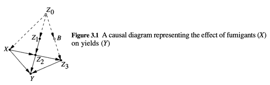screenshot taken from Causality, p.67

• $Z_0$ is last year's eel worm population
• $Z_1$ is the population before the treatment
• $Z_2$ after the treatment
• $Z_3$ at the end of the season
• dashed arrows connect unmeasured quantities, represented as hollow nodes.
• solid arrows connect measured quantities

Note that negative causal assumptions are conveyed through the missing links, e.g. no link between $X$ and $Z_3$ signifies that fumigants do not affect the growth of the surviving eel worms.

Those are domain specific assumptions and our purpose is not to validate or repudiate them but to determine if they are sufficient to quantity the causal effect from non-experimental data (i.e. estimating the total effect of fumigates on yields).

Our end goal is to show that the total effect of $X$ on $Y$ is:

Instead of probabilistic relationships, we can use functional, deterministic relationships:

$x_i = f_i(pa_i, \epsilon_i)$ where:

• $f_i$ are deterministic functions
• $pa_i$ are the parents (causes) of variable $x_i$
• $\epsilon_i$ are mutually independent, random disturbances

The disturbances $\epsilon_i$ represent background factors that the investigator chose not to include. If any of them influences two or more variables - thus violating the independence assumption - that factor must enter the analysis as an unmeasured (latent) variable; e.g. $Z_0$ or $B$ in our example.

The functions $f_i$ and distributions of $\epsilon_i$ will remain unspecified throughout.

Functional representations actually yield the same recursive decomposition of the joint distribution, characteristic of Bayesian networks:

In our example:

External intervention

This is the action of setting a variable $X_i$ to some fixed value $x_i$ and is denoted $\text{do}(X_i=x_i)$.

This amounts to removing the equation $x_i=f_i(pa_i, \epsilon)$ (thus removing the arrows entering $X_i$ on the graph) and substituting $X_i=x_i$ in the remaining equations.

We can then compute the new probability function under the intervention. The causal effect of $X_i$ on $X_j$ is given by $P(x_j\vert\text{do}(X_i=x_i))$ (sometimes noted $P(x_j\vert \hat{x}_i)$ in the book).

Alternatively, we acan represent an intervention as an additional variable $F_i$ in the graph, that takes values $f_i$ (the deterministic functional) or $\text{do}(X_i=x_i)$ (the intervention).

Back to our example. The intervention $\text{do}(X_i=x_i)$ yields the new distribution:

Theorem 3.2.2: Adjusment for direct causes

Let $PA_i$ the set of direct causes (parents) of variable $X_i$. The effect of intervention of $\text{do}(X_i=x_i)$ on $Y$ (any set of variable disjoint of $\{X_i\cup PA_i\}$) is:

We "adjust" for the parents by conditioning on them and weighting by their prior probabilities. This aims at eliminating spurious correlations between cause $X$ and effect $Y$ (some realisations $pa_i$ of variables $PA_i$ might be more probable than other).

Note that we can intervene on multiple variables at once ($\text{do}(S=s)$ where $S$ is some subset of variables).

In summary, given a causal diagram in which all direct causes of intervened variable are observable, we can infer post-intervention distributions from pre-intervention distributions.

In figure 3.1 however, some parents $PA_i$ are unobservable ($Z_0$ and $B$). Next, we will provide graphical tests to determine whether $P(X_j\vert \text{do}(X_i=x_i))$ is estimable.

The back-door criterion (p.79)

First, a reminder on what it means for a variable $Z$ to block a path from $X$ to $Y$.

d-separation or "blocking" (p.16)

A path is a sequence of consecutive edges of any directionality. If a variable (or set of variables) $Z$ blocks the path from $X$ to $Y$, it means that the flow of information is blocked. If we already know $Z$, learning about $X$ won't give us anything about $Y$.

Formally, a path is d-separated or blocked by a set of nodes $Z$ if and only if:

• there is a chain ($X \rightarrow Z \rightarrow Y$) or fork ($X \leftarrow Z \rightarrow Y$) and $Z$ is in the middle.
• there is no inverted fork (or collider) ($X \rightarrow Z \leftarrow Y$) where $Z$ is in the middle.

Basically, a path is blocked by $Z$ iff $X\perp Y | Z$. To understand why a collider breaks this dependency, think about $X=\text{it rains}, Y=\text{the sprinkler is on}, Z=\text{the grass is wet}$. Knowing that the grass is wet but the sprinkler is off helps us deduct that it's raining.

Controlling confounding bias

The book describes Simpson's paradox: "any statistical relationship between two variables may be reversed by including additional factors in the analysis. For example, we may find that students who smoke obtain higher grades than those who do not smoke but, adjusting for age, smokers obtain lower grades in every age groups and, further adjusting for family income, smokers again obtain higher grades than nonsmokers in every income-age group, and so on."

Leaving us with the question, when is adjustment for a given covariate appropriate?

The back-door criterion tells us whether a subset $Z$ of observed variables is sufficient for identifying $P(y\vert do(X)=x)$ where $X$ and $Y$ are observed.

$Z$ satisfies the back-door criterion relative to $X$ and $Y$ if:

• it blocks every path between $X$ and $Y$ containing an arrow into $X$.
• $Z$ contains no descendant of $X$ (because that would mean $X$ has a causal effect on $Z$)

$Z$ is the set of variables that ensure $X$ and $Y$ are d-separated and that are not affected by $X$. We can then change $X$ without affecting the probability of $Y$ (since they are now independent given $Z$).

The causal effect is now given by:

(we adjust for $Z$).

The front-door criterion (p.81)

The first condition of the back-door criterion states that $Z$ should not be impacted by $X$. The front-door criterion tells us that concomitants $Z$ that are impacted by treatment $X$ can be used to facilitate causal inference.

Take the following graph:

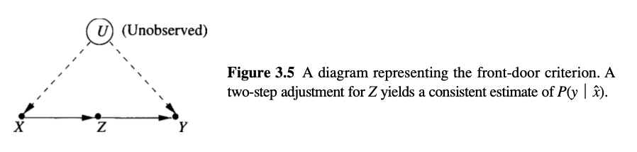
$Z$ does not satisfy the back-door criterion but measurements of $Z$ can enable consistent estimation of $P(y\vert do(X)=x)$.

The joint distribution of the graph is given by:

The intervention $do(X)=x$ removes the factor $P(x\vert u)$ and induces the post-intervention distribution:

Summing over $z$ and $u$:

$u$ is unobserved but we can get rid of it using the conditional independence assumptions encoded in the graph: $P(u\vert z, x)=P(u\vert x)$ and $P(y\vert x,z,u)=P(y\vert z,u)$

Thus:

Finally, we are left with observed quantities only:

This process can be interpreted as a two-step application of the back-door formula:

• first, find the causal effect of $X$ on $Z$, simply $P(z\vert do(X)=x)=P(z\vert x)$ since there is no back-door.
• second, compute the causal effect of $Z$ on $Y$, using $X$ as the concomitant, to block the path $Z\leftarrow X\leftarrow U \rightarrow Y$, giving: $P(y\vert do(Z)=z)=\sum_{x'} P(y\vert x', z)P(x')$

The two effects are then combined using: $P(y\vert do(X)=x)=\sum_z P(y\vert do(Z)=z)P(z\vert do(X)=x)$

Formally, $Z$ satisfies the front-door criterion relative to $X$ and $Y$ if:

1. $Z$ intercepts all directed paths from $X$ to $Y$

2. there is no back-door path from $X$ to $Z$

3. all back-door paths from $Z$ to $Y$ are blocked by $X$

In this case, and if $P(x, z)> 0$ then the causal effect of $X$ on $Y$ is given by:

Q: why the positive distribution requirement?

Possible answer: "we can't infer the effect of action $do(X)=x$ from data in which $X$ never attains the value $x$ in the context wherein the action is applied" (p.78)

"A more powerful symbolic machinery will be introduced in Section 3.4, one that will sidestep algrebraic manipulations such as those used in the derivation of (3.28)".