Source

Calibration: improving our model such that predicted probability distribution is similar to the probability observed in training data.

Calibration plot (=q-q plot)

• 2 classes $\{-1, 1\}$
• sort by predicted probability $\hat p_i = \hat P(y=1 \vert X_i)$
• Define bins $B_i$ between $0$ and $1$ and compute $p_i = \frac{\sum_{k, \hat p_k \in B_i} \mathbb{I}_{y_k =1}}{\lvert B_i \rvert}$
• plot $\hat p_i$ against $\hat p_i$.

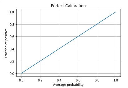
Perfect calibration plot should be identity:

Sigmoid / Platt calibration

Logistic regression on our model output:

$\hat P_\text{new}(y \vert X) = \frac{1}{1 + \exp-[\alpha \hat P(y\vert X) + \beta]}$

Optimized over $\alpha$ and $\beta$.

Isotonic regression

Let $(\hat p_1, p_1), \dots, (\hat p_n, p_n)$. Isotonic regressions seeks weighted least-squares fit $\hat{p_i}^\text{new} \approx p_i$ s.t. $\hat{p_i}^\text{new} \leq \hat{p_j}^\text{new}$ whenever $\hat{p_i} \leq \hat p_j$.

Objective is: $\min \sum_{i=1}^n w_i (\hat p_i^\text{new} - p_i)^2 \text{ s.t. } \hat p_1^\text{new} \leq \dots \leq \hat p_j^\text{new}$ assuming the $p_i$'s are ordered.

This yields a piecewise constant non-decreasing function. To solve this we use the pool adjacent violators algorithm. See these notes.