link to the paper

Contributions:

1. A collision-less hash table used to store embeddings for categorical features in recommender systems (e.g. item id). Includes optimizations such as expirable embeddings and frequency filtering to reduce its memory footprint.

2. a system for online (real-time) training (to mitigate the concept and data drift in recommender systems)

1. collision-less embedding table (cuckoo hash map)

Information from a user's latest interaction is often used as the primary input for training a model. Data is drastically different from that used in conventional deep learning problems like language modeling or computer vision:

1. the features are mostly sparse, categorical and dynamically changing

2. non-stationary distribution (concept drift $p(y\vert X)$ and data-drift $p(X)$)

A common practice is to map sparse, low-frequency categorical features to high dimensional embeddings. However, domain-specific issues arise:

• unlike language models where number of word-pieces (*) is limited, the amount of users and ranking items are orders of magnitude larger. Such an enormous embedding table would hardly fit into a single host memory.
• the embedding table is expected to grow over time as more users and items are admitted.

(*) vocab size is ~32k for monolingual models such as Llama/Mistral and 256k for multi-lingual models such as Google Gemma

Many systems adopt low-collision hashing under the assumptions that:

• collisions are harmless to model quality
• ids are distributed evenly in the embedding table

"monolith consistently outperforms systems that adopts hash-tricks with collisions with roughly similar memory usage, and achieves SOTA online serving AUC"

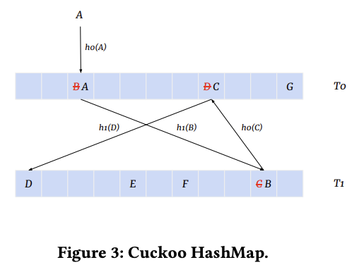
The hash table utilizes a cuckoo hash-map. As depicted in the figure below, it maintains two tables $T_0$ and $T_1$ with different hash functions $h_0$ and $h_1$. When trying to insert an element $A$ into $T_0$, it first attempts to place $A$ at $h_0(A)$. If $h_0(A)$ is occupied by another element $B$, it evicts $B$ from $T_0$ and attempts to insert $B$ at $h_1(B)$ in $T_1$. This process is repeated until either:

• we reach an empty slot and all elements stabilize
• insertion runs into a cycle (e.g. if $B$ was mapped to $h_0(A)$ and $A$ gets mapped to $h_1(B)$) and rehash happens

side note: the rehashing process

When an insertion fails after a maximum number of displacement attempts (indicating a cycle), a full rehash is initiated. 

1. (optional) Enlarge the table: the size of the hash table is increased, often by doubling it, to create more available slots.

2. Generate new hash functions: A new, independent pair of hash functions is selected to provide different mappings for all keys. This is the most critical step, as it breaks the existing cycles.

3. Re-insert all elements: Every existing key from the old table is re-inserted into the newly sized tables using the new hash functions.

If the rehash fails again (which is statistically unlikely but possible), the process is repeated with another set of hash functions

performance

• no collisions
• achieves worst-case $O(1)$ time complexity for look-ups and deletions, and an expected amortized $O(1)$ time complexity for insertions. While a rehash is an expensive operation that takes time proportional to the number of elements, $O(N)$, it happens infrequently. This makes the average, or "amortized," insertion time for cuckoo hashing very efficient, often considered $O(1)$.


good resource on cuckoo hashing: https://cs.stanford.edu/~rishig/courses/ref/l13a.pdf

To avoid blowing up memory, they select which ID to insert:

• IDs are long-tail distributed, where popular IDs occur millions of times while unpopular ones appear no more than ten times. Embeddings corresponding to these infrequent IDs are underfit due to lack of training data. Model quality will not suffer from removal of these IDs with low occurence.
• Stale IDs from a distant history seldom contribute to the current model as many of them are never visited. Thus IDs have a time to live (tunable by embedding table to distinguish features with different sensitivity to historical information)

Note: they mention using a "probabilistic filter to reduce memory usage". Are they referring to a Bloom filter used to check whether the ID is part of set ?

2. real-time training

non-stationary distribution: visual and linguistic patterns barely develop in a time scale of centuries, while the same user interested in one topic could shift their zeal every next minute. as a result, the underlying distribution of user data $p(y|X)$ is non-stationary (concept drift).

To mitigate the effects of concept drift, serving models need to be updated from new user feedback as close to real-time as possible to reflect the latest interest of a user (intuitively, more recent history is a better predictor of the future).

The architecture of monolith follows Tensorflow's distributed Worker-ParameterServer setting:

• worker machines are responsible for performing computations as defined by the graph
• ParameterServer (PS) machines store parameters and updates them according to gradients computed by the workers.

2 stages:

• batch training stage. one epoch only.
• online training stage. The training parameter server periodically synchronizes its parameters to the serving parameter server. Instead of reading a mini-batch from storage (hard disk file storage), the training worker consumes realtime data on-the-fly using the streaming engine described below.


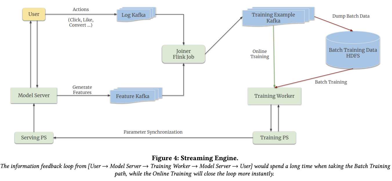
Two Kafka queues:

• one to log user actions (e.g. click on an item)
• one to log features

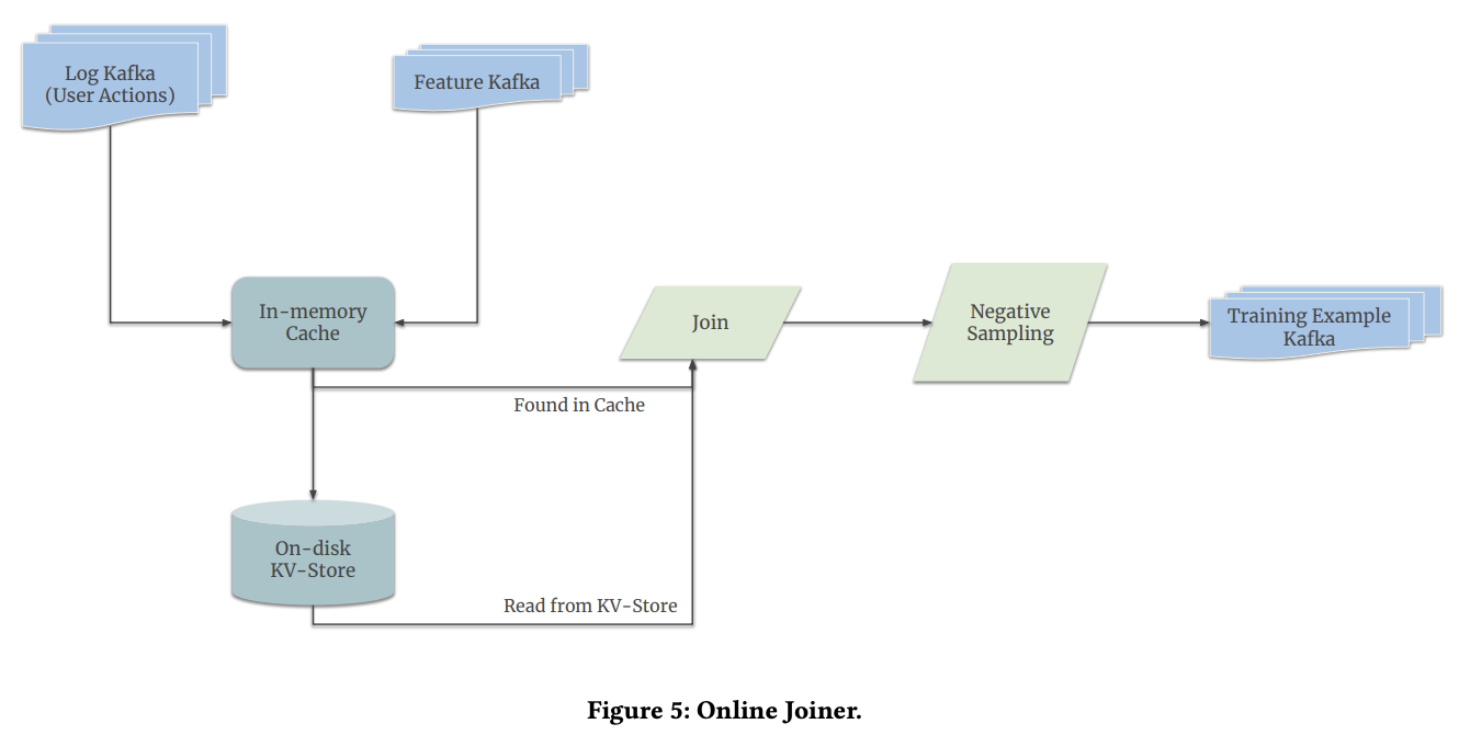
The flink streaming job joins features and labels (online joiner). The produced training tuples are ingested by a third Kafka queue.

For online training, the worker directly reads from the Kafka queue (minute-level intervals)

For batch (offline) training, the data is first dumped to HDFS. After reaching a certain amount, a training worker will fetch mini-batches from HDFS.

User actions and features are fed into the online joiner, with no guarantee in time order. A unique key is used for each request to pair actions to features.

Lag of user actions: a user can take a few days before deciding to buy an item shown days ago. Keeping data for so long would not fit in memory. An on-disk key-value storage is utilized to store features that are waiting for over a certain time period. When a user action log arrives, the system first looks up in the in-memory cache for a feature log, ad then in the key-value storage in case of cache miss.

Negative down-sampling is used to prevent the model from being overwhelmed by negative examples. At serving time, scores are corrected using log-odds correction to prevent a bias towards positives.

Dense parameters are synced less often than sparse parameters (embedding tables). Moreover, they don't sync untouched embedding keys to save on network bandwidth. "Because of momentum-based optimizers, the accumulation of momentum for dense variables is magnified by the gigantic size of recommendation training data, while only a few sparse embeddings receives updates in a single data batch."


fault tolerance: recover a parameter server snapshot. snapshotting a multi-terabyte model incurs large chunks of memory copy and disk I/O. on the other hand, model quality depends on the recency of the snapshot. they settle for daily snapshot, as they notice a tolerable performance degradation.

evaluation:

• they performed an A/B test on their production environment. "Multi-tower architecture, with each tower responsible for learning to predict a specialized kind of user behavior"
• also tested on the Criteo Display Ads Challenge dataset: a large scale standard dataset for benchmarking CTR models.

ID trick

The ID space is $2^{48}$ (e.g. 48 bits).

Decompose ID into a unique remainder and quotient tuple, which each get an embedding table.

i.e. $ID = ID_q \times 2^{24} + ID_r$

i.e. they use two smaller embedding tables instead of one gigantic one. "This effectively reduces embedding table sizes from $2^{48}$ to $2^{25}$". Each id is the sum of two learned vectors.

originally a huge table would have $\text{rows} \times \text{cols} =2^{48}\times d$ parameters.

now you only need: $2\times 2^{24} \times d = 2^{25}$ parameters.

$E$ is not guaranteed to be unique, but the embedding space is so large that collisions are rare (it's a low rank approximation).