This is the Variational Auto-Encoder paper by Kingma & Welling.

For a simple pytorch implementation, check out my github repo, where I auto-encoded CryptoPunks.

Problem statement

There is a random variable $X$ that is generated by:

• sampling a latent variable $z\sim p_{\theta^*}(z)$
• sampling $x\sim p_{\theta^*}(x\vert z)$

where the true parameters $\theta^*$ of the distribution and the latent variable $z$ are hidden.

Reminder on the evidence lower bound

Suppose that we want to estimate the distribution $p_{\theta^*}$ by estimating parameters $\theta$. $\theta$ is both used to generate $z$ and then $x$ (by sampling $p_\theta{x\vert z}$).

Let's say we found some appropriate $\theta$, it's intractable to estimate $p_\theta(x)$ for a given $x$ because we need to marginalize over all $z$s:

$p_\theta(x)=\int p_\theta(x\vert z)p_\theta(z)dz$

However, we also know that, given a certain $z$ we have: $p_\theta(x,z) = p_\theta(x/vert z)p(z)$ and $p_\theta(x, z) = p_\theta(z\vert x)p(x)$.

Combining the two:

$p_\theta(x)=p_\theta(z)p_\theta(x\vert z)/p_\theta(z\vert x)$ for any $z$.

If we can find a good approximation of $p_\theta(z\vert x)$, we can compute $p_\theta(x)$. However:

• we might not have a closed form solution
• $p_\theta(z\vert x) = p_\theta(x\vert z)p_\theta(z)/p_\theta(x)$ and we already established that $p(x)$ is intractable.

Therefore, we'll use another distribution family $q_\phi(z\vert x)$ to approximate $p_\theta(z\vert x)$.

Now, to estimate the best model $p_\theta$ we wish to maximize it's likelihood, which is the probability density function: $p_\theta(x)$. For convenience, we usually use the log-likelihood. The optimization problem is equivalent since $\log$ is a monotonously increasing function.

$\ln p_\theta(x) = \ln \int p_\theta(x, z)dz$

Recall that this is intractable, because of the integral over $z$. We can estimate this using importance sampling:

$\ln p_\theta(x) = \ln \mathbb{E}_{q_\phi(z\vert x)}\frac{p_\theta(x, z)}{q_\phi(z\vert x)} \geq \mathbb{E}_{q_\phi(z\vert x)}\ln\frac{p_\theta(x, z)}{q_\phi(z\vert x)}\text{ (Jensen's inequality)}$

Now, this term: $\mathbb{E}_{q_\phi(z\vert x)}\ln\frac{p_\theta(x, z)}{q_\phi(z\vert x)}$ is what we call the evidence lower bound $\mathcal{L}(\theta, \phi)$. But it's not over. Let's put it on the left hand side and combine it with the log-likelihood term $\ln p_\theta(x)$:

$\ln p_\theta(x) - \mathbb{E}_{q_\phi(z\vert x)}\ln\frac{p_\theta(x, z)}{q_\phi(z\vert x)} \geq 0$

where

$\begin{aligned}\ln p_\theta(x) - \mathbb{E}_{q_\phi(z\vert x)}\ln\frac{p_\theta(x, z)}{q_\phi(z\vert x)} & = -\mathbb{E}_{q_\phi(z\vert x)}[\ln\frac{p_\theta(x, z)}{q_\phi(z\vert x)} - \ln p_\theta(x)] \\& = -\mathbb{E}_{q_\phi(z\vert x)}[\ln\frac{p_\theta(x, z)/p_\theta(x)}{q_\phi(z\vert x)}] \\& = -\mathbb{E}_{q_\phi(z\vert x)}[\ln\frac{p_\theta(z\vert x)}{q_\phi(z\vert x)}] \\& = D_{KL}(q_\phi(z\vert x)\Vert p_\theta(z\vert x)) \\\end{aligned}$

So we basically have:

$\underbrace{\ln p_\theta(x)}_{\text{log likelihood}} - \underbrace{\mathcal{L}(\theta, \phi)}_{\text{ELBO}} = \underbrace{D_{KL}(q_\phi(z\vert x)\Vert p_\theta(z\vert x))}_{\text{KL divergence}} \geq 0$

Therefore, by maximizing the ELBO we are maximizing the log-likelihood. The point of the paper is to find a way to differentiate and optimize the ELBO with low variance.

To recap, here's our encoder: $q_\phi(z\vert x)\approx p_\theta(z\vert x)$; here's our decoder $p_\theta(x\vert z)$. We'll learn $\phi$ and $\theta$ jointly.

We want the algo to work in the case of:

• intractibility: can't compute $p_\theta(z) = \int p_\theta(z)p_\theta(x\vert z)dz$ or $p_\theta(z\vert x)=\frac{p_\theta(x\vert z)p_\theta(z)}{p_\theta(x)}$ (EM can't be used). $p_\theta(x)$ intractable because of large dimensionality (image). $p_\theta(x\vert z)$ intractable due to large number of hidden variables (in case of neural net with nonlinear hidden layer for example).
• large dataset: monte carlo EM would be too slow (expensive sampling loop per datapoint)

Some relevant applications:

• the parameters $\theta$ can be of interest if we're analyzing some natural process or want to generate artificial data (by sampling $p(x\vert \theta)$). We want efficient max likelihood (maximize probability of seeing the data given the model) or max à priori estimation (maximize probability of the model given the data; requires a model prior) of parameters $\theta$.
• representing data (e.g. generating image embeddings): posterior inference of $z$ given $x$
• marginal inference of $x$ for tasks where a prior over $x$ is required like image denoising, inpainting, superresolution

Stochastic Gradient Variational Bayes

The ELBO $L(p_\theta, q_\phi)$ can also be written as $L(p_\theta, q_\phi)=-D_{KL}(q_\phi(z\vert x)\lVert p_\theta(z)) + \mathbb{E_{q_\phi(z\vert x)}}(\log p_\theta(x\vert z))$

The first term is the KL divergence which can be seen as a regularization term with respect to the prior $p_\theta(z)$. The second term is the reconstruction loss: given $z$ we want to reconstruct $x$.

Naively, we can use a monte carlo gradient estimator for either term: $\nabla_\phi \mathbb{E}_{q_\phi(z)}[f(z)]=\nabla_\phi \int_z q(z)f(z)dz=\int_z \nabla_\phi q(z) f(z) dz =\int_z q(z)\underbrace{\frac{1}{q(z)}\nabla_\phi q(z)}_{\nabla_\phi \log q_\phi(z)} f(z) dz = \mathbb{E}[f(z)\nabla_\phi \log q_\phi(z)]$

where $f(z) = \log\frac{p_\theta(z)}{q_\phi(z\vert x)}$ or $f(z)=\log p_\theta(x\vert z)$

Thus: $\nabla_\phi \mathbb{E}_{q_\phi(z)}[f(z)] \approx \frac{1}{L}\sum f(z)\nabla_\phi \log q_\phi(z)$

However, this estimator has very high variance.

We can reparameterize $q_\phi(z\vert x)$ as $\tilde z = g_\phi(\epsilon , x), \epsilon\sim p(\epsilon)$.

For instance, $z=\mathcal{N}(\mu, \sigma)$: $\tilde z=\mu + \sigma \epsilon, \epsilon\sim\mathcal{N}(0, 1)$

$\mathbb{E}_{q_\phi(z\vert x)}[f(z)]=\mathbb{E}_{p(\epsilon)}[f(g_\phi(\epsilon, x))]\approx \frac{1}{L}\sum f(g_\phi(\epsilon, x))$

KL divergence can be integrated analytically (e.g. when prior $p_\theta(z)$ and posterior $q_\phi(z\vert x)$ are gaussian, see appendix B in the paper). KL divergence can be interpreted as regularization to encourage $q(x\vert z)$ to be close to prior. Only the expected reconstruction error requires estimation $\mathbb{E}_{q_\phi(z\vert x)}[\log p_\theta(x\vert z)]$

Example: Variational Auto-Encoder

• we set a prior over the latent $p_\theta(z)=\mathcal{N}(z; 0, I)$.
• For discrete data, encoder $p_\theta(x\vert z)$ is a multivariate Bernoulli distribution:

$\log p(x\vert z) = \sum x_i \log y_i + (1-x_i)\log(1-y_i)$

(product of each pixel independently, $p(x_i\vert z) = y_i$ if $x_i=1$ and $1-y_i$ otherwise)

where $y_i=\text{sigmoid}(W_2 + \tanh(W_1 z +b_1) + b_2)$

• For real value data, encoder $p_\theta(x\vert z)$ is a multivariate gaussian:

$\log p(x\vert z) = \log \mathcal{N}(x; \mu, \sigma^2 I)$

where $\mu=W_1 h + b_1, \log \sigma^2 = W_2 h + b_2, h =\tanh(W_0 z + b_0)$.

• The true posterior $p_\theta(z\vert x)$ is intractable. We approximate it with decoder $q_\phi(z\vert x)$. For $q_\phi(z\vert x)$, same formula as multivar gaussian (with diff parameters) and $z$ and $x$ are swapped

KL divergence can be computed and differentiated analytically. For reconstruction loss, we sample $z\sim \mu + \sigma \epsilon$ where $\epsilon\sim\mathcal{N}(0,I)$.

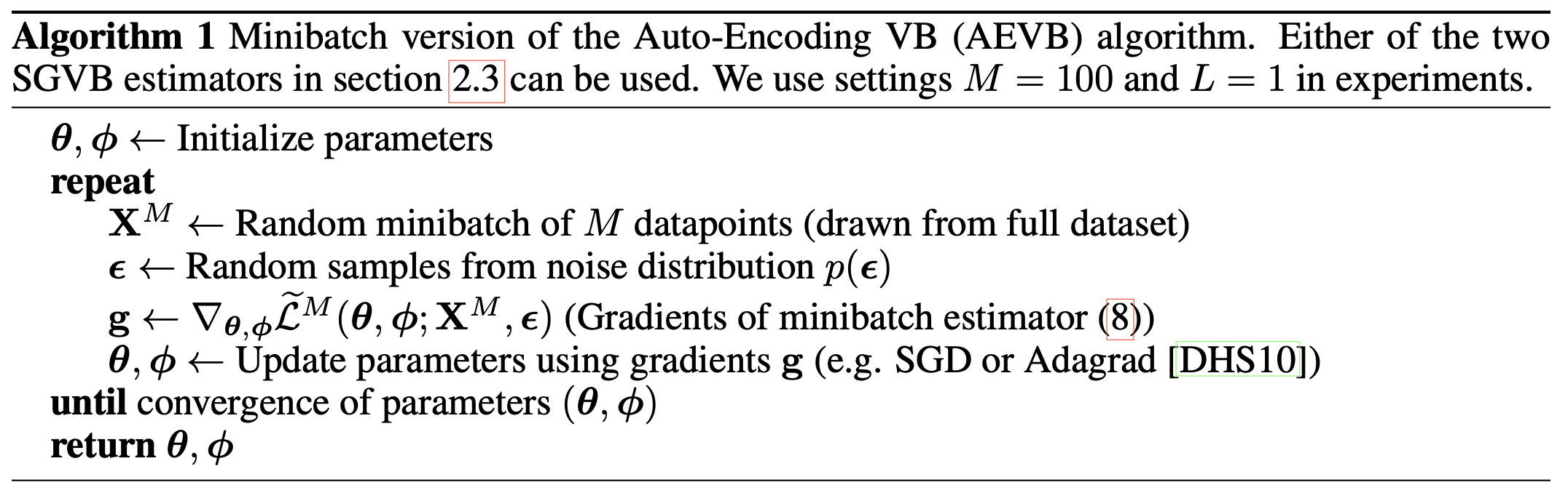
AEVB algorithm: